
Causal Inference:
The Mixtape.
Buy the print version today:
Buy the print version today:
\[ % Define terms \newcommand{\Card}{\text{Card }} \DeclareMathOperator*{\cov}{cov} \DeclareMathOperator*{\var}{var} \DeclareMathOperator{\Var}{Var\,} \DeclareMathOperator{\Cov}{Cov\,} \DeclareMathOperator{\Prob}{Prob} \newcommand{\independent}{\perp \!\!\! \perp} \DeclareMathOperator{\Post}{Post} \DeclareMathOperator{\Pre}{Pre} \DeclareMathOperator{\Mid}{\,\vert\,} \DeclareMathOperator{\post}{post} \DeclareMathOperator{\pre}{pre} \]
One of the most important tools in the causal inference toolkit is the panel data estimator. The estimators are designed explicitly for longitudinal data—the repeated observing of a unit over time. Under certain situations, repeatedly observing the same unit over time can overcome a particular kind of omitted variable bias, though not all kinds. While it is possible that observing the same unit over time will not resolve the bias, there are still many applications where it can, and that’s why this method is so important. We review first the DAG describing just such a situation, followed by discussion of a paper, and then present a data set exercise in R and Stata.1
Before I dig into the technical assumptions and estimation methodology for panel data techniques, I want to review a simple DAG illustrating those assumptions. This DAG comes from Imai and Kim (2017). Let’s say that we have data on a column of outcomes \(Y_i\), which appear in three time periods. In other words, \(Y_{i1}\), \(Y_{i2}\), and \(Y_{i3}\) where \(i\) indexes a particular unit and \(t=1,2,3\) index the time period where each \(i\) unit is observed. Likewise, we have a matrix of covariates, \(D_i\), which also vary over time—\(D_{i1}\), \(D_{i2}\), and \(D_{i3}\). And finally, there exists a single unit-specific unobserved variable, \(u_i\), which varies across units, but which does not vary over time for that unit. Hence the reason that there is no \(t=1,2,3\) subscript for our \(u_i\) variable. Key to this variable is (a) it is unobserved in the data set, (b) it is unit-specific, and (c) it does not change over time for a given unit \(i\). Finally there exists some unit-specific time-invariant variable, \(X_i\). Notice that it doesn’t change over time, just \(u_i\), but unlike \(u_i\) it is observed.
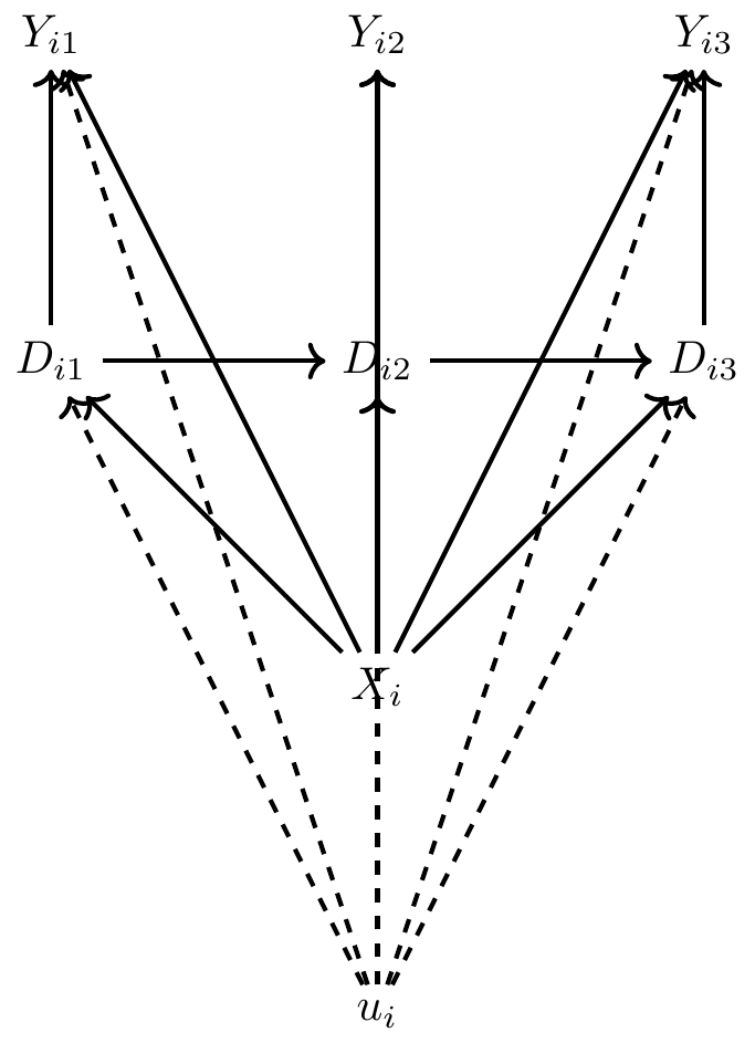
As this is the busiest DAG we’ve seen so far, it merits some discussion. First, let us note that \(D_{i1}\) causes both \(Y_{i1}\) as well as the next period’s treatment value, \(D_{i2}\). Second, note that an unobserved confounder, \(u_i\), determines all \(Y\) and \(D\) variables. Consequently, \(D\) is endogenous since \(u_i\) is unobserved and absorbed into the structural error term of the regression model. Thirdly, there is no time-varying unobserved confounder correlated with \(D_{it}\)—the only confounder is \(u_i\), which we call the unobserved heterogeneity. Fourth, past outcomes do not directly affect current outcomes (i.e., no direct edge between the \(Y_{it}\) variables). Fifth, past outcomes do not directly affect current treatments (i.e., no direct edge from \(Y_{i, t-1}\) to \(D_{it}\)). And finally, past treatments, \(D_{i,t-1}\) do not directly affect current outcomes, \(Y_{it}\) (i.e., no direct edge from \(D_{i,t-1}\) and \(Y_{it}\)). It is under these assumptions that we can use a particular panel method called fixed effects to isolate the causal effect of \(D\) on \(Y\).2
What might an example of this be? Let’s return to our story about the returns to education. Let’s say that we are interested in the effect of schooling on earnings, and schooling is partly determined by unchanging genetic factors which themselves determine unobserved ability, like intelligence, contentiousness, and motivation (Conley and Fletcher 2017). If we observe the same people’s time-varying earnings and schoolings over time, then if the situation described by the above DAG describes both the directed edges and the missing edges, then we can use panel fixed effects models to identify the causal effect of schooling on earnings.
When we use the term “panel data,” what do we mean? We mean a data set where we observe the same units (e.g., individuals, firms, countries, schools) over more than one time period. Often our outcome variable depends on several factors, some of which are observed and some of which are unobserved in our data, and insofar as the unobserved variables are correlated with the treatment variable, then the treatment variable is endogenous and correlations are not estimates of a causal effect. This chapter focuses on the conditions under which a correlation between \(D\) and \(Y\) reflects a causal effect even with unobserved variables that are correlated with the treatment variable. Specifically, if these omitted variables are constant over time, then even if they are heterogeneous across units, we can use panel data estimators to consistently estimate the effect of our treatment variable on outcomes.
There are several different kinds of estimators for panel data, but we will in this chapter only cover two: pooled ordinary least squares (POLS) and fixed effects (FE).3
First we need to set up our notation. With some exceptions, panel methods are usually based on the traditional notation and not the potential outcomes notation.
Let \(Y\) and \(D\equiv(D_1, D_2, \dots, D_k)\) be observable random variables and \(u\) be an unobservable random variable. We are interested in the partial effects of variable \(D_j\) in the population regression function: \[ E\big[Y\mid D_1,D_2, \dots , D_k, u\big] \] We observe a sample of \(i=1,2,\dots,N\) cross-sectional units for \(t=1,2,\dots,T\) time periods (a balanced panel). For each unit \(i\), we denote the observable variables for all time periods as \(\{(Y_{it},D_{it}):t=1,2,\dots,T\}\).4 Let \(D_{it}\equiv(D_{it1},D_{it2}, \dots, D_{itk})\) be a \(1\times K\) vector. We typically assume that the actual cross-sectional units (e.g., individuals in a panel) are identical and independent draws from the population in which case \(\{Y_i, D_i, u_i\}^N_{i=1}\sim i.i.d.\), or cross-sectional independence. We describe the main observables, then, as \(Y_i \equiv (Y_{i1}, Y_{i2}, \dots, Y_{iT})'\) and \(D_i \equiv (D_{i1},D_{i2}, \dots, D_{iT})\).
It’s helpful now to illustrate the actual stacking of individual units across their time periods. A single unit \(i\) will have multiple time periods \(t\) \[ Y_i=\left( \begin{array}{c} Y_{i1} \\ \vdots \\ Y_{it} \\ \vdots \\ Y_{iT} \end{array} \right)_{T\times 1} \qquad D_i = \left( \begin{array}{ccccc} D_{i,1,1} & D_{i,1,2} & D_{i,1,j} & \dots & D_{i,1,K} \\ \vdots & \vdots & \vdots & & \vdots \\ D_{i,t,1} & D_{i,t,2} & D_{i,t,j} & \dots & D_{i,t,K} \\ \vdots & \vdots & \vdots & & \vdots \\ D_{i,T,1} & D_{i,T,2} & D_{i,T,j} & \dots & D_{i,T,K} \end{array} \right)_{T\times K} \] And the entire panel itself with all units included will look like this: \[ Y = \left( \begin{array}{c} Y_{1} \\ \vdots \\ Y_{i} \\ \vdots \\ Y_{N} \end{array} \right)_{NT\times 1} \qquad D = \left( \begin{array}{c} D_1 \\ \vdots \\ D_i \\ \vdots \\ D_N \end{array} \right)_{NT \times K} \] For a randomly drawn cross-sectional unit \(i\), the model is given by \[ Y_{it}=\delta D_{it}+u_i+\varepsilon_{it}, \quad t=1,2,\dots,T \] As always, we use our schooling-earnings example for motivation. Let \(Y_{it}\) be log earnings for a person \(i\) in year \(t\). Let \(D_{it}\) be schooling for person \(i\) in year \(t\). Let \(\delta\) be the returns to schooling. Let \(u_i\) be the sum of all time-invariant person-specific characteristics, such as unobserved ability. This is, as I said earlier, often called the unobserved heterogeneity. And let \(\varepsilon_{it}\) be the time-varying unobserved factors that determine a person’s wage in a given period. This is often called the idiosyncratic error. We want to know what happens when we regress \(Y_{it}\) on \(D_{it}\).
The first estimator we will discuss is the pooled ordinary least squares, or POLS estimator. When we ignore the panel structure and regress \(Y_{it}\) on \(D_{it}\) we get \[ Y_{it}=\delta D_{it} + \eta_{it}; \quad t=1,2,\dots,T \] with composite error \(\eta_{it} \equiv c_i + \varepsilon_{it}\). The main assumption necessary to obtain consistent estimates for \(\delta\) is: \[ E\big[\eta_{it}\mid D_{i1},D_{i2}, \dots, D_{iT}\big] = E\big[\eta_{it}\mid D_{it}\big] = 0 \quad \text{for $t=1,2,\dots, T$} \] While our DAG did not include \(\varepsilon_{it}\), this would be equivalent to assuming that the unobserved heterogeneity, \(c_i\), was uncorrelated with \(D_{it}\) for all time periods.
But this is not an appropriate assumption in our case because our DAG explicitly links the unobserved heterogeneity to both the outcome and the treatment in each period. Or using our schooling-earnings example, schooling is likely based on unobserved background factors, \(u_i\), and therefore without controlling for it, we have omitted variable bias and \(\widehat{\delta}\) is biased. No correlation between \(D_{it}\) and \(\eta_{it}\) necessarily means no correlation between the unobserved \(u_i\) and \(D_{it}\) for all \(t\) and that is just probably not a credible assumption. An additional problem is that \(\eta_{it}\) is serially correlated for unit \(i\) since \(u_i\) is present in each \(t\) period. And thus heteroskedastic robust standard errors are also likely too small.
Let’s rewrite our unobserved effects model so that this is still firmly in our minds: \[ Y_{it} = \delta D_{it} + u_i + \varepsilon_{it}; \quad t=1,2,\dots,T \] If we have data on multiple time periods, we can think of \(u_i\) as fixed effects to be estimated. OLS estimation with fixed effects yields \[ \big(\widehat{\delta}, \widehat{u}_1, \dots, \widehat{u}_N\big) = \underset{b,m_1,\dots,m_N}{\arg\min} \sum_{i=1}^N\sum_{t=1}^T (Y_{it}-D_{it}b- m_i)^2 \] which amounts to including \(N\) individual dummies in regression of \(Y_{it}\) on \(D_{it}\).
The first-order conditions (FOC) for this minimization problem are: \[ \sum_{i=1}^N \sum_{t=1}^T D_{it}' \big(Y_{it} - D_{it}\widehat{\delta} - \widehat{u}_i\big)=0 \] and \[ \sum_{t=1}^T\big(Y_{it} - D_{it}\widehat{\delta} - \widehat{u}_i\big)=0 \] for \(i=1,\dots,N\).
Therefore, for \(i=1, \dots, N\), \[ \widehat{u}_i = \dfrac{1}{T} \sum_{t=1}^T\big(Y_{it}-D_{it}\widehat{\delta}\big)= \overline{Y}_i-\overline{D}_i\widehat{\delta}, \] where \[ \overline{D}_i \equiv \dfrac{1}{T}\sum_{t=1}^TD_{it}; \bar{Y}_i \equiv \dfrac{1}{T} \sum_{t=1}^T Y_{it} \] Plug this result into the first FOC to obtain: \[ \begin{gathered} \widehat{\delta} = \bigg( \sum_{i=1}^N \sum_{t=1}^T (D_{it} - \overline{D}_i)'(D_{it} - \overline{D}_i) \bigg)^{-1} \bigg( \sum_{i=1}^N \sum_{t=1}^T (D_{it} - \overline{D}_i)'(Y_{it} - \overline{Y})\bigg) \\ \widehat{\delta} = \bigg(\sum_{i=1}^N \sum_{t=1}^T \ddot{D}_{it}'\ddot{D}_{it} \bigg)^{-1} \bigg( \sum_{i=1}^N \sum_{t=1}^T \ddot{D}_{it}' \ddot{Y}_{it} \bigg)\end{gathered} \] with time-demeaned variables \(\ddot{D}_{it} \equiv D_{it}-\overline{D},\ddot{Y}_{it} \equiv Y_{it} - \overline{Y}_i\).
In case it isn’t clear, though, running a regression with the time-demeaned variables \(\ddot{Y}_{it}\equiv Y_{it} - \overline{Y}_i\) and \(\ddot{D}_{it} \equiv D_{it} - \overline{D}\) is numerically equivalent to a regression of \(Y_{it}\) on \(D_{it}\) and unit-specific dummy variables. Hence the reason this is sometimes called the “within” estimator, and sometimes called the “fixed effects” estimator. And when year fixed effects are included, the “twoway fixed effects” estimator. They are the same thing.5
Even better, the regression with the time-demeaned variables is consistent for \(\delta\) even when \(C[D_{it},u_i]\ne 0\) because time-demeaning eliminates the unobserved effects. Let’s see this now:
\[ \begin{align} Y_{it} & =\delta D_{it} + u_i + \varepsilon_{it} \\ \overline{Y}_i & =\delta \overline{D}_i + u_i + \overline{\varepsilon}_{i} \\ (Y_{it} - \overline{Y}_i) & =(\delta D_{it} - \delta\overline{D}) + (u_i - u_i) + (\varepsilon_{it} - \overline{\varepsilon}_i) \\ \ddot{Y}_{it} & =\delta\ddot{D}_{it}+\ddot{\varepsilon}_{it} \end{align} \]
Where’d the unobserved heterogeneity go?! It was deleted when we time-demeaned the data. And as we said, including individual fixed effects does this time demeaning automatically so that you don’t have to go to the actual trouble of doing it yourself manually.6
So how do we precisely do this form of estimation? There are three ways to implement the fixed effects (within) estimator. They are:
Demean and regress \(\ddot{Y}_{it}\) on \(\ddot{D}_{it}\) (need to correct degrees of freedom).
Regress \(Y_{it}\) on \(D_{it}\) and unit dummies (dummy variable regression).
Regress \(Y_{it}\) on \(D_{it}\) with canned fixed effects routine in Stata or R.
Later in this chapter, I will review an example from my research. We will estimate a model involving sex workers using pooled OLS, a FE, and a demeaned OLS model. I’m hoping this exercise will help you see the similarities and differences across all three approaches.
We kind of reviewed the assumptions necessary to identify \(\delta\) with our fixed effects (within) estimator when we walked through that original DAG, but let’s supplement that DAG intuition with some formality. The main identification assumptions are:
\(E[\varepsilon_{it}\mid D_{i1}, D_{i2}, \dots, D_{iT}, u_i]=0; t=1,2,\dots,T\)
This means that the regressors are strictly exogenous conditional on the unobserved effect. This allows \(D_{it}\) to be arbitrarily related to \(u_i\), though. It only concerns the relationship between \(D_{it}\) and \(\varepsilon_{it}\), not \(D_{it}\)’s relationship to \(u_i\).
\(rank\bigg( \sum_{t=1}^T E[\ddot{D}_{it}'\ddot{D}_{it}]\bigg) = K\)
It shouldn’t be a surprise to you by this point that we have a rank condition, because even when we were working with the simpler linear models, the estimated coefficient was always a scaled covariance, where the scaling was by a variance term. Thus regressors must vary over time for at least some \(i\) and not be collinear in order that \(\widehat{\delta} \approx \delta\).
The properties of the estimator under assumptions 1 and 2 are that \(\widehat{\delta}_{FE}\) is consistent (\(\underset{N\rightarrow \infty}{p\lim}\ \widehat{\delta}_{FE,N}=\delta\)) and \(\widehat{\delta}_{FE}\) is unbiased conditional on D.
I only briefly mention inference. But the standard errors in this framework must be “clustered” by panel unit (e.g., individual) to allow for correlation in the \(\varepsilon_{it}\) for the same person \(i\) over time. This yields valid inference so long as the number of clusters is “large.”7
But, there are still things that fixed effects (within) estimators cannot solve. For instance, let’s say we regressed crime rates onto police spending per capita. Becker (1968) argues that increases in the probability of arrest, usually proxied by police per capita or police spending per capita, will reduce crime. But at the same time, police spending per capita is itself a function of crime rates. This kind of reverse causality problem shows up in most panel models when regressing crime rates onto police. For instance, see Cornwell and Trumbull (1994). I’ve reproduced a portion of this in Table 8.1. The dependent variable is crime rates by county in North Carolina for a panel, and they find a positive correlation between police and crime rates, which is the opposite of what Becker predicts. Does this mean having more police in an area causes higher crime rates? Or does it likely reflect the reverse causality problem?
| Dependent variable | Between | Within | 2SLS (FE) | 2SLS (No FE) |
|---|---|---|---|---|
| Police | 0.364 | 0.413 | 0.504 | 0.419 |
| (0.060) | (0.027) | (0.617) | (0.218) | |
| Controls | Yes | Yes | Yes | Yes |
North Carolina county level data. Standard errors in parenthesis.
So, one situation in which you wouldn’t want to use panel fixed effects is if you have reverse causality or simultaneity bias. And specifically when that reverse causality is very strong in observational data. This would technically violate the DAG, though, that we presented at the start of the chapter. Notice that if we had reverse causality, then \(Y \rightarrow D\), which is explicitly ruled out by this theoretical model contained in the DAG. But obviously, in the police—crime example, that DAG would be inappropriate, and any amount of reflection on the problem should tell you that that DAG is inappropriate. Thus it requires, as I’ve said repeatedly, some careful reflection, and writing out exactly what the relationship is between the treatment variables and the outcome variables in a DAG can help you develop a credible identification strategy.
The second situation in which panel fixed effects don’t buy you anything is if the unobserved heterogeneity is time-varying. In this situation, the demeaning has simply demeaned an unobserved time-variant variable, which is then moved into the composite error term, and which since time-demeaned \(\ddot{u}_{it}\) correlated with \(\ddot{D}_{it}\), \(\ddot{D}_{it}\) remains endogenous. Again, look carefully at the DAG—panel fixed effects are only appropriate if \(u_i\) is unchanging. Otherwise it’s just another form of omitted variable bias. So, that said, don’t just blindly use fixed effects and think that it solves your omitted variable bias problem—in the same way that you shouldn’t use matching just because it’s convenient to do. You need a DAG, based on an actual economic model, which will allow you to build the appropriate research design. Nothing substitutes for careful reasoning and economic theory, as they are the necessary conditions for good research design.
When might this be true? Let’s use an example from Cornwell and Rupert (1997) in which the authors attempt to estimate the causal effect of marriage on earnings. It’s a well-known stylized fact that married men earn more than unmarried men, even controlling for observables. But the question is whether that correlation is causal, or whether it reflects unobserved heterogeneity (i.e., selection bias).
So let’s say that we had panel data on individuals. These individuals \(i\) are observed for four periods \(t\). We are interested in the following equation:8 \[ Y_{it}=\alpha+\delta M_{it}+\beta X_{it}+A_{i} +\gamma_i+\varepsilon_{it} \] Let the outcome be their wage \(Y_{it}\) observed in each period, and which changes each period. Let wages be a function of marriage. Since people’s marital status changes over time, the marriage variable is allowed to change value over time. But race and gender, in most scenarios, do not ordinarily change over time; these are variables which are ordinarily unchanging, or what you may sometimes hear called “time invariant.” Finally, the variables \(A_i\) and \(\gamma_i\) are variables which are unobserved, vary cross-sectionally across the sample, but do not vary over time. I will call these measures of unobserved ability, which may refer to any fixed endowment in the person, like fixed cognitive ability or noncognitive ability such as “grit.” The key here is that it is unit-specific, unobserved, and time-invariant. The \(\varepsilon_{it}\) is the unobserved determinants of wages which are assumed to be uncorrelated with marriage and other covariates.
Cornwell and Rupert (1997) estimate both a feasible generalized least squares model and three fixed effects models (each of which includes different time-varying controls). The authors call the fixed effects regression a “within” estimator, because it uses the within unit variation for eliminating the confounding. Their estimates are presented in Table 8.2.
| Dependent variable | FGLS | Within | Within | Within |
|---|---|---|---|---|
| Married | 0.083 | 0.056 | 0.051 | 0.033 |
| (0.022) | (0.026) | (0.026) | (0.028) | |
| Education controls | Yes | No | No | No |
| Tenure | No | No | Yes | Yes |
| Quadratics in years married | No | No | No | Yes |
Standard errors in parenthesis.
Notice that the FGLS (column 1) finds a strong marriage premium of around 8.3%. But, once we begin estimating fixed effects models, the effect gets smaller and less precise. The inclusion of marriage characteristics, such as years married and job tenure, causes the coefficient on marriage to fall by around 60% from the FGLS estimate, and is no longer statistically significant at the 5% level.
Next I’d like to introduce a Stata exercise based on data collection for my own research: a survey of sex workers. You may or may not know this, but the Internet has had a profound effect on sex markets. It has moved sex work indoors while simultaneously breaking the traditional link between sex workers and pimps. It has increased safety and anonymity, too, which has had the effect of causing new entrants. The marginal sex worker has more education and better outside options than traditional US sex workers (Cunningham and Kendall 2011, 2014, 2016). The Internet, in sum, caused the marginal sex worker to shift towards women more sensitive to detection, harm, and arrest.
In 2008 and 2009, I surveyed (with Todd Kendall) approximately 700 US Internet-mediated sex workers. The survey was a basic labor-market survey; I asked them about their illicit and legal labor-market experiences, and about demographics. The survey had two parts: a “static” provider-specific section and a “panel” section. The panel section asked respondents to share information about each of the previous four sessions with clients.9
I have created a shortened version of the data set and uploaded it to Github. It includes a few time-invariant provider characteristics, such as race, age, marital status, years of schooling, and body mass index, as well as several time-variant session-specific characteristics including the log of the hourly price, the log of the session length (in hours), characteristics of the client himself, whether a condom was used in any capacity during the session, whether the client was a “regular,” etc.
In this exercise, you will estimate three types of models: a pooled OLS model, a fixed effects (FE), and a demeaned OLS model. The model will be of the following form:
\[ \begin{align} Y_{is} & =\beta_i X_i + \gamma_{is} Z_{is} + u_i + \varepsilon_{is} \\ \ddot{Y}_{is} & = \gamma_{is} \ddot{Z}_{is} + \ddot \eta_{is} \end{align} \]
where \(u_i\) is both unobserved and correlated with \(Z_{is}\).
The first regression model will be estimated with pooled OLS and the second model will be estimated using both fixed effects and OLS. In other words, I’m going to have you estimate the model using canned routines in Stata and R with individual fixed effects, as well as demean the data manually and estimate the demeaned regression using OLS.
Notice that the second regression has a different notation on the dependent and independent variable; it represents the fact that the variables are columns of demeaned variables. Thus \(\ddot Y_{is} = Y_{is} - \overline{Y}_i\). Secondly, notice that the time-invariant \(X_i\) variables are missing from the second equation. Do you understand why that is the case? These variables have also been demeaned, but since the demeaning is across time, and since these time-invariant variables do not change over time, the demeaning deletes them from the expression. Notice, also, that the unobserved individual specific heterogeneity, \(u_i\), has disappeared. It has disappeared for the same reason that the \(X_i\) terms are gone—because the mean of \(u_i\) over time is itself, and thus the demeaning deletes it.
Let’s examine these models using the following R and Stata programs.
use https://github.com/scunning1975/mixtape/raw/master/sasp_panel.dta, clear
tsset id session
foreach x of varlist lnw age asq bmi hispanic black other asian schooling cohab married divorced separated age_cl unsafe llength reg asq_cl appearance_cl provider_second asian_cl black_cl hispanic_cl othrace_cl hot massage_cl
drop if `x'==.
bysort id: gen s=_N
keep if s==4
foreach x of varlist lnw age asq bmi hispanic black other asian schooling cohab married divorced separated age_cl unsafe llength reg asq_cl appearance_cl provider_second asian_cl black_cl hispanic_cl  othrace_cl hot massage_cl

egen mean_`x'=mean(`x'), by(id)
gen demean_`x'=`x' - mean_`x'
drop mean*

xi: reg lnw  age asq bmi hispanic black other asian schooling cohab married divorced separated age_cl unsafe llength reg asq_cl appearance_cl provider_second asian_cl black_cl hispanic_cl othrace_cl hot massage_cl, robust
xi: xtreg lnw  age asq bmi hispanic black other asian schooling cohab married divorced separated age_cl unsafe llength reg asq_cl appearance_cl provider_second asian_cl black_cl hispanic_cl othrace_cl hot massage_cl, fe i(id) robust
reg demean_lnw demean_age demean_asq demean_bmi demean_hispanic demean_black demean_other demean_asian demean_schooling demean_cohab demean_married demean_divorced demean_separated demean_age_cl demean_unsafe demean_llength demean_reg demean_asq_cl demean_appearance_cl demean_provider_second demean_asian_cl demean_black_cl demean_hispanic_cl demean_othrace_cl demean_hot demean_massage_cl, robust cluster(id)library(tidyverse)
library(haven)
library(estimatr)
library(plm)
read_data <- function(df)
{
full_path <- paste("https://github.com/scunning1975/mixtape/raw/master/",
df, sep = "")
df <- read_dta(full_path)
return(df)
}
sasp <- read_data("sasp_panel.dta")
#-- Delete all NA
sasp <- na.omit(sasp)
#-- order by id and session
sasp <- sasp %>%
arrange(id, session)
#Balance Data
balanced_sasp <- make.pbalanced(sasp,
balance.type = "shared.individuals")
#Demean Data
balanced_sasp <- balanced_sasp %>% mutate(
demean_lnw = lnw - ave(lnw, id),
demean_age = age - ave(age, id),
demean_asq = asq - ave(asq, id),
demean_bmi = bmi - ave(bmi, id),
demean_hispanic = hispanic - ave(hispanic, id),
demean_black = black - ave(black, id),
demean_other = other - ave(other, id),
demean_asian = asian - ave(asian, id),
demean_schooling = schooling - ave(schooling, id),
demean_cohab = cohab - ave(cohab, id),
demean_married = married - ave(married, id),
demean_divorced = divorced - ave(divorced, id),
demean_separated = separated - ave(separated, id),
demean_age_cl = age_cl - ave(age_cl, id),
demean_unsafe = unsafe - ave(unsafe, id),
demean_llength = llength - ave(llength, id),
demean_reg = reg - ave(reg, id),
demean_asq_cl = asq_cl - ave(asq_cl, id),
demean_appearance_cl = appearance_cl - ave(appearance_cl, id),
demean_provider_second = provider_second - ave(provider_second, id),
demean_asian_cl = asian_cl - ave(asian_cl, id),
demean_black_cl = black_cl - ave(black_cl, id),
demean_hispanic_cl = hispanic_cl - ave(hispanic_cl, id),
demean_othrace_cl = othrace_cl - ave(othrace_cl, id),
demean_hot = hot - ave(hot, id),
demean_massage_cl = massage_cl - ave(massage_cl, id)
)
#-- POLS
ols <- lm_robust(lnw ~ age + asq + bmi + hispanic + black + other + asian + schooling + cohab + married + divorced + separated +
age_cl + unsafe + llength + reg + asq_cl + appearance_cl + provider_second + asian_cl + black_cl + hispanic_cl +
othrace_cl + hot + massage_cl, data = balanced_sasp)
summary(ols)
#-- FE
formula <- as.formula("lnw ~ age + asq + bmi + hispanic + black + other + asian + schooling +
cohab + married + divorced + separated +
age_cl + unsafe + llength + reg + asq_cl + appearance_cl +
provider_second + asian_cl + black_cl + hispanic_cl +
othrace_cl + hot + massage_cl")
model_fe <- lm_robust(formula = formula,
data = balanced_sasp,
fixed_effect = ~id,
se_type = "stata")
summary(model_fe)
#-- Demean OLS
dm_formula <- as.formula("demean_lnw ~ demean_age + demean_asq + demean_bmi +
demean_hispanic + demean_black + demean_other +
demean_asian + demean_schooling + demean_cohab +
demean_married + demean_divorced + demean_separated +
demean_age_cl + demean_unsafe + demean_llength + demean_reg +
demean_asq_cl + demean_appearance_cl +
demean_provider_second + demean_asian_cl + demean_black_cl +
demean_hispanic_cl + demean_othrace_cl +
demean_hot + demean_massage_cl")
ols_demean <- lm_robust(formula = dm_formula,
data = balanced_sasp, clusters = id,
se_type = "stata")
summary(ols_demean)import numpy as np
import pandas as pd
import statsmodels.api as sm
import statsmodels.formula.api as smf
from itertools import combinations
import plotnine as p
# read data
import ssl
ssl._create_default_https_context = ssl._create_unverified_context
def read_data(file):
return pd.read_stata("https://github.com/scunning1975/mixtape/raw/master/" + file)
sasp = read_data("sasp_panel.dta")
#-- Delete all NA
sasp = sasp.dropna()
#-- order by id and session
sasp.sort_values('id', inplace=True)
#Balance Data
times = len(sasp.session.unique())
in_all_times = sasp.groupby('id')['session'].apply(lambda x : len(x)==times).reset_index()
in_all_times.rename(columns={'session':'in_all_times'}, inplace=True)
balanced_sasp = pd.merge(in_all_times, sasp, how='left', on='id')
balanced_sasp = balanced_sasp[balanced_sasp.in_all_times]
balanced_sasp.shape
provider_second = np.zeros(balanced_sasp.shape[0])
provider_second[balanced_sasp.provider_second == "2. Yes"] = 1
balanced_sasp.provider_second = provider_second
#Demean Data
features = balanced_sasp.columns.to_list()
features = [x for x in features if x not in ['session', 'id', 'in_all_times']]
demean_features = ["demean_{}".format(x) for x in features]
balanced_sasp[demean_features] = balanced_sasp.groupby('id')[features].apply(lambda x : x - np.mean(x))
##### Pooled OLS
dep_var = "+".join(features)
formula = """lnw ~ age + asq + bmi + hispanic + black + other + asian + schooling + cohab +
married + divorced + separated + age_cl + unsafe + llength + reg + asq_cl +
appearance_cl + provider_second + asian_cl + black_cl + hispanic_cl +
othrace_cl + hot + massage_cl"""
ols = sm.OLS.from_formula(formula, data=balanced_sasp).fit()
ols.summary()
# #### Fixed Effects
balanced_sasp['y'] = balanced_sasp.lnw
formula = """lnw ~ -1 + C(id) + age + asq + bmi + hispanic + black + other + asian + schooling +
cohab + married + divorced + separated +
age_cl + unsafe + llength + reg + asq_cl + appearance_cl +
provider_second + asian_cl + black_cl + hispanic_cl +
othrace_cl + hot + massage_cl"""
ols = sm.OLS.from_formula(formula, data=balanced_sasp).fit(cov_type='cluster',
cov_kwds={'groups': balanced_sasp['id']})
ols.summary()
# #### Demean OLS
#-- Demean OLS
dm_formula = """demean_lnw ~ demean_age + demean_asq + demean_bmi +
demean_hispanic + demean_black + demean_other +
demean_asian + demean_schooling + demean_cohab +
demean_married + demean_divorced + demean_separated +
demean_age_cl + demean_unsafe + demean_llength + demean_reg +
demean_asq_cl + demean_appearance_cl +
demean_provider_second + demean_asian_cl + demean_black_cl +
demean_hispanic_cl + demean_othrace_cl +
demean_hot + demean_massage_cl"""
ols = sm.OLS.from_formula(dm_formula, data=balanced_sasp).fit(cov_type='cluster', cov_kwds={'groups': balanced_sasp['id']})
ols.summary() A few comments about this analysis. Some of the respondents left certain questions blank, most likely due to concerns about anonymity and privacy. So I dropped anyone who had missing values for the sake of this exercise. This leaves us with a balanced panel. I have organized the output into Table 8.3. There’s a lot of interesting information in these three columns, some of which may surprise you if only for the novelty of the regressions. So let’s talk about the statistically significant ones. The pooled OLS regressions, recall, do not control for unobserved heterogeneity, because by definition those are unobservable. So these are potentially biased by the unobserved heterogeneity, which is a kind of selection bias, but we will discuss them anyhow.
| Depvar: | POLS | FE | Demeaned OLS |
|---|---|---|---|
| Unprotected sex with client of any kind | 0.013 | 0.051\(^{*}\) | 0.051\(^{*}\) |
| (0.028) | (0.028) | (0.026) | |
| Ln(Length) | \(-0.308^{***}\) | \(-0.435^{***}\) | \(-0.435^{***}\) |
| (0.028) | (0.024) | (0.019) | |
| Client was a Regular | \(-0.047\)\(^{*}\) | \(-0.037^{**}\) | \(-0.037^{**}\) |
| (0.028) | (0.019) | (0.017) | |
| Age of Client | \(-0.001\) | 0.002 | 0.002 |
| (0.009) | (0.007) | (0.006) | |
| Age of Client Squared | 0.000 | \(-0.000\) | \(-0.000\) |
| (0.000) | (0.000) | (0.000) | |
| Client Attractiveness (Scale of 1 to 10) | 0.020\(^{***}\) | 0.006 | 0.006 |
| (0.007) | (0.006) | (0.005) | |
| Second Provider Involved | 0.055 | 0.113\(^{*}\) | 0.113\(^{*}\) |
| (0.067) | (0.060) | (0.048) | |
| Asian Client | \(-0.014\) | \(-0.010\) | \(-0.010\) |
| (0.049) | (0.034) | (0.030) | |
| Black Client | 0.092 | 0.027 | 0.027 |
| (0.073) | (0.042) | (0.037) | |
| Hispanic Client | 0.052 | \(-0.062\) | \(-0.062\) |
| (0.080) | (0.052) | (0.045) | |
| Other Ethnicity Client | 0.156\(^{**}\) | 0.142\(^{***}\) | 0.142\(^{***}\) |
| (0.068) | (0.049) | (0.045) | |
| Met Client in Hotel | 0.133\(^{***}\) | 0.052\(^{*}\) | 0.052\(^{*}\) |
| (0.029) | (0.027) | (0.024) | |
| Gave Client a Massage | \(-0.134^{***}\) | \(-0.001\) | \(-0.001\) |
| (0.029) | (0.028) | (0.024) | |
| Age of provider | 0.003 | 0.000 | 0.000 |
| (0.012) | (.) | (.) | |
| Age of provider squared | \(-0.000\) | 0.000 | 0.000 |
| (0.000) | (.) | (.) | |
| Body Mass Index | \(-0.022^{***}\) | 0.000 | 0.000 |
| (0.002) | (.) | (.) | |
| Hispanic | \(-0.226^{***}\) | 0.000 | 0.000 |
| (0.082) | (.) | (.) | |
| Black | 0.028 | 0.000 | 0.000 |
| (0.064) | (.) | (.) | |
| Other | \(-0.112\) | 0.000 | 0.000 |
| (0.077) | (.) | (.) | |
| Asian | 0.086 | 0.000 | 0.000 |
| (0.158) | (.) | (.) | |
| Imputed Years of Schooling | 0.020\(^{**}\) | 0.000 | 0.000 |
| (0.010) | (.) | (.) | |
| Cohabitating (living with a partner) but unmarried | \(-0.054\) | 0.000 | 0.000 |
| (0.036) | (.) | (.) | |
| Currently married and living with your spouse | 0.005 | 0.000 | 0.000 |
| (0.043) | (.) | (.) | |
| Divorced and not remarried | \(-0.021\) | 0.000 | 0.000 |
| (0.038) | (.) | (.) | |
| Married but not currently living with your spouse | \(-0.056\) | 0.000 | 0.000 |
| (0.059) | (.) | (.) | |
| N | 1,028 | 1,028 | 1,028 |
| Mean of dependent variable | 5.57 | 5.57 | 0.00 |
Heteroskedastic robust standard errors in parenthesis clustered at the provider level. \(^{*}\)\(p<0.10\), \(^{**}\)\(p<0.05\), \(^{**}\)\(^{*}\)\(p<0.01\)
First, a simple scan of the second and third column will show that the fixed effects regression which included (not shown) dummies for the individual herself is equivalent to a regression on the demeaned data. This should help persuade you that the fixed effects and the demeaned (within) estimators are yielding the same coefficients.
But second, let’s dig into the results. One of the first things we observe is that in the pooled OLS model, there is not a compensating wage differential detectable on having unprotected sex with a client.10 But, notice that in the fixed effects model, unprotected sex has a premium. This is consistent with Rosen (1986) who posited the existence of risk premia, as well as Gertler, Shah, and Bertozzi (2005) who found risk premia for sex workers using panel data. Gertler, Shah, and Bertozzi (2005), though, find a much larger premia of over 20% for unprotected sex, whereas I am finding only a mere 5%. This could be because a large number of the unprotected instances are fellatio, which carries a much lower risk of infection than unprotected receptive intercourse. Nevertheless, it is interesting that unprotected sex, under the assumption of strict exogeneity, appears to cause wages to rise by approximately 5%, which is statistically significant at the 10% level. Given an hourly wage of $262, this amounts to a mere 13 additional dollars per hour. The lack of a finding in the pooled OLS model seems to suggest that the unobserved heterogeneity was masking the effect.
Next we look at the session length. Note that I have already adjusted the price the client paid for the length of the session so that the outcome is a log wage, as opposed to a log price. As this is a log-log regression, we can interpret the coefficient on log length as an elasticity. When we use fixed effects, the elasticity increases from \(-0.308\) to \(-0.435\). The significance of this result, in economic terms, though, is that there appear to be “volume discounts” in sex work. That is, longer sessions are more expensive, but at a decreasing rate. Another interesting result is whether the client was a “regular,” which meant that she had seen him before in another session. In our pooled OLS model, regulars paid 4.7% less, but this shrinks slightly in our fixed effects model to 3.7% reductions. Economically, this could be lower because new clients pose risks that repeat customers do not pose. Thus, if we expect prices to move closer to marginal cost, the disappearance of some of the risk from the repeated session should lower price, which it appears to do.
Another factor related to price is the attractiveness of the client. Interestingly, this does not go in the direction we may have expected. One might expect that the more attractive the client, the less he pays. But in fact it is the opposite. Given other research that finds beautiful people earn more money (Hamermesh and Biddle 1994), it’s possible that sex workers are price-discriminating. That is, when they see a handsome client, they deduce he earns more, and therefore charge him more. This result does not hold up when including fixed effects, though, suggesting that it is due to unobserved heterogeneity, at least in part.
Similar to unprotected sex, a second provider present has a positive effect on price, which is only detectable in the fixed effects model. Controlling for unobserved heterogeneity, the presence of a second provider increases prices by 11.3%. We also see that she discriminates against clients of “other” ethnicities, who pay 14.2% more than White clients. There’s a premium associated with meeting in a hotel which is considerably smaller when controlling for provider fixed effects by almost a third. This positive effect, even in the fixed effects model, may simply represent the higher costs associated with meeting in a hotel room. The other coefficients are not statistically significant.
Many of the time-invariant results are also interesting, though. For instance, perhaps not surprisingly, women with higher BMI earn less. Hispanics earn less than White sex workers. And women with more schooling earn more, something which is explored in greater detail in Cunningham and Kendall (2016).
In conclusion, we have been exploring the usefulness of panel data for estimating causal effects. We noted that the fixed effects (within) estimator is a very useful method for addressing a very specific form of endogeneity, with some caveats. First, it will eliminate any and all unobserved and observed time-invariant covariates correlated with the treatment variable. So long as the treatment and the outcome varies over time, and there is strict exogeneity, then the fixed effects (within) estimator will identify the causal effect of the treatment on some outcome.
But this came with certain qualifications. For one, the method couldn’t handle time-variant unobserved heterogeneity. It’s thus the burden of the researcher to determine which type of unobserved heterogeneity problem they face, but if they face the latter, then the panel methods reviewed here are not unbiased and consistent. Second, when there exists strong reverse causality pathways, then panel methods are biased. Thus, we cannot solve the problem of simultaneity, such as what Wright faced when estimating the price elasticity of demand, using the fixed effects (within) estimator. Most likely, we are going to have to move into a different framework when facing that kind of problem.
Still, many problems in the social sciences may credibly be caused by a time-invariant unobserved heterogeneity problem, in which case the fixed effects (within) panel estimator is useful and appropriate.
Buy the print version today:
There’s a second reason to learn this estimator. Some of these estimators, such as linear models with time and unit fixed effects, are the modal estimators used in difference-in-differences.↩︎
The fixed-effects estimator, when it includes year fixed effects, is popularly known as the “twoway fixed effects” estimator.↩︎
A common third type of panel estimator is the random effects estimator, but in my experience, I have used it less often than fixed effects, so I decided to omit it. Again, this is not because it is unimportant. I just have chosen to do fewer things in more detail based on whether I think they qualify as the most common methods used in the present period by applied empiricists. See Wooldridge (2010) for a more comprehensive treatment, though, of all panel methods including random effects.↩︎
For simplicity, I’m ignoring the time-invariant observations, \(X_i\) from our DAG for reasons that will hopefully soon be made clear.↩︎
One of the things you’ll find over time is that things have different names, depending on the author and tradition, and those names are often completely uninformative.↩︎
Though feel free to do it if you want to convince yourself that they are numerically equivalent, probably just starting with a bivariate regression for simplicity.↩︎
In my experience, when an econometrician is asked how large is large, they say “the size of your data.” But that said, there is a small clusters literature and usually it’s thought that fewer than thirty clusters is too small (as a rule of thumb). So it may be that having around thirty to forty clusters is sufficient for the approaching of infinity. This will usually hold in most panel applications such as US states or individuals in the NSLY, etc.↩︎
We use the same notation as used in their paper, as opposed to the \(\ddot{Y}\) notation presented earlier.↩︎
Technically, I asked them to share about the last five sessions, but for this exercise, I have dropped the fifth due to low response rates on the fifth session.↩︎
There were three kinds of sexual encounter—vaginal receptive sex, anal receptive sex, and fellatio. Unprotected sex is coded as any sex act without a condom.↩︎