3  Directed Acyclic Graphs

Causal Inference:
The Mixtape.

Buy the print version today:

Buy from Amazon Buy from Yale Press

The history of graphical causal modeling goes back to the early twentieth century and Sewall Wright, one of the fathers of modern genetics and son of the economist Philip Wright. Sewall developed path diagrams for genetics, and Philip, it is believed, adapted them for econometric identification (Matsueda 2012).¹

But despite that promising start, the use of graphical modeling for causal inference has been largely ignored by the economics profession, with a few exceptions (J. Heckman and Pinto 2015; Imbens 2019). It was revitalized for the purpose of causal inference when computer scientist and Turing Award winner Judea Pearl adapted them for his work on artificial intelligence. He explained this in his magnum opus, which is a general theory of causal inference that expounds on the usefulness of his directed graph notation (Pearl 2009). Since graphical models are immensely helpful for designing a credible identification strategy, I have chosen to include them for your consideration. Let’s review graphical models, one of Pearl’s contributions to the theory of causal inference.²

3.1 Introduction to DAG Notation

Using directed acyclic graphical (DAG) notation requires some up-front statements. The first thing to notice is that in DAG notation, causality runs in one direction. Specifically, it runs forward in time. There are no cycles in a DAG. To show reverse causality, one would need to create multiple nodes, most likely with two versions of the same node separated by a time index. Similarly, simultaneity, such as in supply and demand models, is not straightforward with DAGs (J. Heckman and Pinto 2015). To handle either simultaneity or reverse causality, it is recommended that you take a completely different approach to the problem than the one presented in this chapter. Third, DAGs explain causality in terms of counterfactuals. That is, a causal effect is defined as a comparison between two states of the world—one state that actually happened when some intervention took on some value and another state that didn’t happen (the “counterfactual”) under some other intervention.

Think of a DAG as like a graphical representation of a chain of causal effects. The causal effects are themselves based on some underlying, unobserved structured process, one an economist might call the equilibrium values of a system of behavioral equations, which are themselves nothing more than a model of the world. All of this is captured efficiently using graph notation, such as nodes and arrows. Nodes represent random variables, and those random variables are assumed to be created by some data-generating process.³ Arrows represent a causal effect between two random variables moving in the intuitive direction of the arrow. The direction of the arrow captures the direction of causality.

Causal effects can happen in two ways. They can either be direct (e.g., \(D \rightarrow Y\)), or they can be mediated by a third variable (e.g., \(D \rightarrow X \rightarrow Y\)). When they are mediated by a third variable, we are capturing a sequence of events originating with \(D\), which may or may not be important to you depending on the question you’re asking.

A DAG is meant to describe all causal relationships relevant to the effect of \(D\) on \(Y\). What makes the DAG distinctive is both the explicit commitment to a causal effect pathway and the complete commitment to the lack of a causal pathway represented by missing arrows. In other words, a DAG will contain both arrows connecting variables and choices to exclude arrows. And the lack of an arrow necessarily means that you think there is no such relationship in the data—this is one of the strongest beliefs you can hold. A complete DAG will have all direct causal effects among the variables in the graph as well as all common causes of any pair of variables in the graph.

At this point, you may be wondering where the DAG comes from. It’s an excellent question. It may be the question. A DAG is supposed to be a theoretical representation of the state-of-the-art knowledge about the phenomena you’re studying. It’s what an expert would say is the thing itself, and that expertise comes from a variety of sources. Examples include economic theory, other scientific models, conversations with experts, your own observations and experiences, literature reviews, as well as your own intuition and hypotheses.

I have included this material in the book because I have found DAGs to be useful for understanding the critical role that prior knowledge plays in identifying causal effects. But there are other reasons too. One, I have found that DAGs are very helpful for communicating research designs and estimators if for no other reason than pictures speak a thousand words. This is, in my experience, especially true for instrumental variables, which have a very intuitive DAG representation. Two, through concepts such as the backdoor criterion and collider bias, a well-designed DAG can help you develop a credible research design for identifying the causal effects of some intervention. As a bonus, I also think a DAG provides a bridge between various empirical schools, such as the structural and reduced form groups. And finally, DAGs drive home the point that assumptions are necessary for any and all identification of causal effects, which economists have been hammering at for years (Wolpin 2013).

3.1.1 A simple DAG

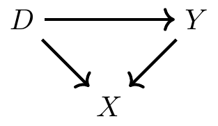
Let’s begin with a simple DAG to illustrate a few basic ideas. I will expand on it to build slightly more complex ones later.

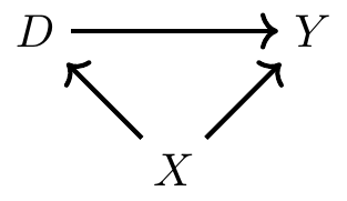
In this DAG, we have three random variables: \(X\), \(D\), and \(Y\). There is a direct path from \(D\) to \(Y\), which represents a causal effect. That path is represented by \(D \rightarrow Y\). But there is also a second path from \(D\) to \(Y\) called the backdoor path. The backdoor path is \(D \leftarrow X \rightarrow Y\). While the direct path is a causal effect, the backdoor path is not causal. Rather, it is a process that creates spurious correlations between \(D\) and \(Y\) that are driven solely by fluctuations in the \(X\) random variable.

The idea of the backdoor path is one of the most important things we can learn from the DAG. It is similar to the notion of omitted variable bias in that it represents a variable that determines the outcome and the treatment variable. Just as not controlling for a variable like that in a regression creates omitted variable bias, leaving a backdoor open creates bias. The backdoor path is \(D \leftarrow X \rightarrow Y\). We therefore call \(X\) a confounder because it jointly determines \(D\) and \(Y\), and so confounds our ability to discern the effect of \(D\) on \(Y\) in naı̈ve comparisons.

Think of the backdoor path like this: Sometimes when \(D\) takes on different values, \(Y\) takes on different values because \(D\) causes \(Y\). But sometimes \(D\) and \(Y\) take on different values because \(X\) takes on different values, and that bit of the correlation between \(D\) and \(Y\) is purely spurious. The existence of two causal pathways is contained within the correlation between \(D\) and \(Y\).

Let’s look at a second DAG, which is subtly different from the first. In the previous example, \(X\) was observed. We know it was observed because the direct edges from \(X\) to \(D\) and \(Y\) were solid lines. But sometimes there exists a confounder that is unobserved, and when there is, we represent its direct edges with dashed lines. Consider the following DAG:

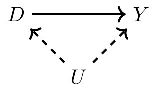
Same as before, \(U\) is a noncollider along the backdoor path from \(D\) to \(Y\), but unlike before, \(U\) is unobserved to the researcher. It exists, but it may simply be missing from the data set. In this situation, there are two pathways from \(D\) to \(Y\). There’s the direct pathway, \(D \rightarrow Y\), which is the causal effect, and there’s the backdoor pathway, \(D \leftarrow U \rightarrow Y\). And since \(U\) is unobserved, that backdoor pathway is open.

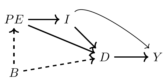
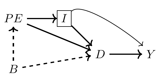
Let’s now move to another example, one that is slightly more realistic. A classical question in labor economics is whether college education increases earnings. According to the Becker human capital model (Becker 1994), education increases one’s marginal product, and since workers are paid their marginal product in competitive markets, education also increases their earnings. But college education is not random; it is optimally chosen given an individual’s subjective preferences and resource constraints. We represent that with the following DAG. As always, let \(D\) be the treatment (e.g., college education) and \(Y\) be the outcome of interest (e.g., earnings). Furthermore, let \(PE\) be parental education, \(I\) be family income, and \(B\) be unobserved background factors, such as genetics, family environment, and mental ability.

This DAG is telling a story. And one of the things I like about DAGs is that they invite everyone to listen to the story together. Here is my interpretation of the story being told. Each person has some background. It’s not contained in most data sets, as it measures things like intelligence, contentiousness, mood stability, motivation, family dynamics, and other environmental factors—hence, it is unobserved in the picture. Those environmental factors are likely correlated between parent and child and therefore subsumed in the variable \(B\).

Background causes a child’s parent to choose her own optimal level of education, and that choice also causes the child to choose their level of education through a variety of channels. First, there is the shared background factors, \(B\). Those background factors cause the child to choose a level of education, just as her parent had. Second, there’s a direct effect, perhaps through simple modeling of achievement or setting expectations, a kind of peer effect. And third, there’s the effect that parental education has on family earnings, \(I\), which in turn affects how much schooling the child receives. Family earnings may itself affect the child’s future earnings through bequests and other transfers, as well as external investments in the child’s productivity.

This is a simple story to tell, and the DAG tells it well, but I want to alert your attention to some subtle points contained in this DAG. The DAG is actually telling two stories. It is telling what is happening, and it is telling what is not happening. For instance, notice that \(B\) has no direct effect on the child’s earnings except through its effect on schooling. Is this realistic, though? Economists have long maintained that unobserved ability both determines how much schooling a child gets and directly affects the child’s future earnings, insofar as intelligence and motivation can influence careers. But in this DAG, there is no relationship between background and earnings, which is itself an assumption. And you are free to call foul on this assumption if you think that background factors affect both schooling and the child’s own productivity, which itself should affect wages. So what if you think that there should be an arrow from \(B\) to \(Y\)? Then you would draw one and rewrite all the backdoor paths between \(D\) and \(Y\).

Now that we have a DAG, what do we do? I like to list out all direct and indirect paths (i.e., backdoor paths) between \(D\) and \(Y\). Once I have all those, I have a better sense of where my problems are. So:

1. \(D \rightarrow Y\) (the causal effect of education on earnings)

2. \(D \leftarrow I \rightarrow Y\) (backdoor path 1)

3. \(D \leftarrow PE \rightarrow I \rightarrow Y\) (backdoor path 2)

4. \(D \leftarrow B \rightarrow PE \rightarrow I \rightarrow Y\) (backdoor path 3)

So there are four paths between \(D\) and \(Y\): one direct causal effect (which arguably is the important one if we want to know the return on schooling) and three backdoor paths. And since none of the variables along the backdoor paths is a collider, each of the backdoors paths is open. The problem, though, with open backdoor paths is that they create systematic and independent correlations between \(D\) and \(Y\). Put a different way, the presence of open backdoor paths introduces bias when comparing educated and less-educated workers.

3.1.2 Colliding

But what is this collider? It’s an unusual term, one you may have never seen before, so let’s introduce it with another example. I’m going to show you what a collider is graphically using a simple DAG, because it’s an easy thing to see and a slightly more complicated phenomenon to explain. So let’s work with a new DAG. Pay careful attention to the directions of the arrows, which have changed.

As before, let’s list all paths from \(D\) to \(Y\):

1. \(D \rightarrow Y\) (causal effect of \(D\) on \(Y\))

2. \(D \rightarrow X \leftarrow Y\) (backdoor path 1)

Just like last time, there are two ways to get from \(D\) to \(Y\). You can get from \(D\) to \(Y\) using the direct (causal) path, \(D \rightarrow Y\). Or you can use the backdoor path, \(D \rightarrow X \leftarrow Y\). But something is different about this backdoor path; do you see it? This time the \(X\) has two arrows pointing to it, not away from it. When two variables cause a third variable along some path, we call that third variable a “collider.” Put differently, \(X\) is a collider along this backdoor path because \(D\) and the causal effects of \(Y\) collide at \(X\). But so what? What makes a collider so special? Colliders are special in part because when they appear along a backdoor path, that backdoor path is closed simply because of their presence. Colliders, when they are left alone, always close a specific backdoor path.

3.1.3 Backdoor criterion

We care about open backdoor paths because they create systematic, noncausal correlations between the causal variable of interest and the outcome you are trying to study. In regression terms, open backdoor paths introduce omitted variable bias, and for all you know, the bias is so bad that it flips the sign entirely. Our goal, then, is to close these backdoor paths. And if we can close all of the otherwise open backdoor paths, then we can isolate the causal effect of \(D\) on \(Y\) using one of the research designs and identification strategies discussed in this book. So how do we close a backdoor path?

There are two ways to close a backdoor path. First, if you have a confounder that has created an open backdoor path, then you can close that path by conditioning on the confounder. Conditioning requires holding the variable fixed using something like subclassification, matching, regression, or another method. It is equivalent to “controlling for” the variable in a regression. The second way to close a backdoor path is the appearance of a collider along that backdoor path. Since colliders always close backdoor paths, and conditioning on a collider always opens a backdoor path, choosing to ignore the colliders is part of your overall strategy to estimate the causal effect itself. By not conditioning on a collider, you will have closed that backdoor path and that takes you closer to your larger ambition to isolate some causal effect.

When all backdoor paths have been closed, we say that you have come up with a research design that satisfies the backdoor criterion. And if you have satisfied the backdoor criterion, then you have in effect isolated some causal effect. But let’s formalize this: a set of variables \(X\) satisfies the backdoor criterion in a DAG if and only if \(X\) blocks every path between confounders that contain an arrow from \(D\) to \(Y\). Let’s review our original DAG involving parental education, background and earnings.

The minimally sufficient conditioning strategy necessary to achieve the backdoor criterion is the control for \(I\), because \(I\) appeared as a noncollider along every backdoor path (see earlier). It might literally be no simpler than to run the following regression: \[ Y_i = \alpha + \delta D_i + \beta I_i + \varepsilon_i \] By simply conditioning on \(I\), your estimated \(\widehat{\delta}\) takes on a causal interpretation.⁴

But maybe in hearing this story, and studying it for yourself by reviewing the literature and the economic theory surrounding it, you are skeptical of this DAG. Maybe this DAG has really bothered you from the moment you saw me produce it because you are skeptical that \(B\) has no relationship to \(Y\) except through \(D\) or \(PE\). That skepticism leads you to believe that there should be a direct connection from \(B\) to \(Y\), not merely one mediated through own education.

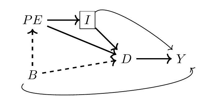
Note that including this new backdoor path has created a problem because our conditioning strategy no longer satisfies the backdoor criterion. Even controlling for \(I\), there still exist spurious correlations between \(D\) and \(Y\) due to the \(D \leftarrow B \rightarrow Y\) backdoor path. Without more information about the nature of \(B \rightarrow Y\) and \(B \rightarrow D\), we cannot say much more about the partial correlation between \(D\) and \(Y\). We just are not legally allowed to interpret \(\widehat{\delta}\) from our regression as the causal effect of \(D\) on \(Y\).

3.1.4 More examples of collider bias

The issue of conditioning on a collider is important, so how do we know if we have that problem or not? No data set comes with a flag saying “collider” and “confounder.” Rather, the only way to know whether you have satisfied the backdoor criterion is with a DAG, and a DAG requires a model. It requires in-depth knowledge of the data-generating process for the variables in your DAG, but it also requires ruling out pathways. And the only way to rule out pathways is through logic and models. There is no way to avoid it—all empirical work requires theory to guide it. Otherwise, how do you know if you’ve conditioned on a collider or a noncollider? Put differently, you cannot identify treatment effects without making assumptions.

In our earlier DAG with collider bias, we conditioned on some variable \(X\) that was a collider—specifically, it was a descendent of \(D\) and \(Y\). But that is just one example of a collider. Oftentimes, colliders enter into the system in very subtle ways. Let’s consider the following scenario: Again, let \(D\) and \(Y\) be child schooling and child future earnings. But this time we introduce three new variables—\(U1\), which is father’s unobserved genetic ability; \(U2\), which is mother’s unobserved genetic ability; and \(I\), which is joint family income. Assume that \(I\) is observed but that \(U_i\) is unobserved for both parents.

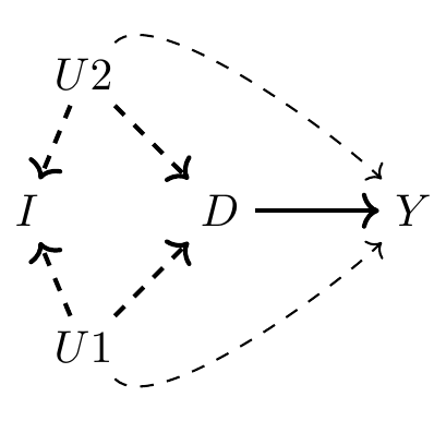
Notice in this DAG that there are several backdoor paths from \(D\) to \(Y\). They are as follows:

1. \(D \leftarrow U2 \rightarrow Y\)

2. \(D \leftarrow U1 \rightarrow Y\)

3. \(D \leftarrow U1 \rightarrow I \leftarrow U2 \rightarrow Y\)

4. \(D \leftarrow U2 \rightarrow I \leftarrow U1 \rightarrow Y\)

Notice, the first two are open-backdoor paths, and as such, they cannot be closed, because \(U1\) and \(U2\) are not observed. But what if we controlled for \(I\) anyway? Controlling for \(I\) only makes matters worse, because it opens the third and fourth backdoor paths, as \(I\) was a collider along both of them. It does not appear that any conditioning strategy could meet the backdoor criterion in this DAG. And any strategy controlling for \(I\) would actually make matters worse. Collider bias is a difficult concept to understand at first, so I’ve included a couple of examples to help you sort through it.

Causal Inference:
The Mixtape.

Buy the print version today:

Buy from Amazon Buy from Yale Press

3.1.5 Discrimination and collider bias

Let’s examine a real-world example around the problem of gender discrimination in labor-markets. It is common to hear that once occupation or other characteristics of a job are conditioned on, the wage disparity between genders disappears or gets smaller. For instance, critics once claimed that Google systematically underpaid its female employees. But Google responded that its data showed that when you take “location, tenure, job role, level and performance” into consideration, women’s pay is basically identical to that of men. In other words, controlling for characteristics of the job, women received the same pay.

But what if one of the ways gender discrimination creates gender disparities in earnings is through occupational sorting? If discrimination happens via the occupational match, then naïve contrasts of wages by gender controlling for occupation characteristics will likely understate the presence of discrimination in the marketplace. Let me illustrate this with a DAG based on a simple occupational sorting model with unobserved heterogeneity.

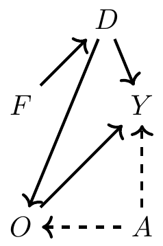
Notice that there is in fact no effect of female gender on earnings; women are assumed to have productivity identical to that of men. Thus, if we could control for discrimination, we’d get a coefficient of zero as in this example because women are, initially, just as productive as men.⁵

But in this example, we aren’t interested in estimating the effect of being female on earnings; we are interested in estimating the effect of discrimination itself. Now you can see several noticeable paths between discrimination and earnings. They are as follows:

1. \(D \rightarrow O \rightarrow Y\)

2. \(D \rightarrow O \leftarrow A \rightarrow Y\)

The first path is not a backdoor path; rather, it is a path whereby discrimination is mediated by occupation before discrimination has an effect on earnings. This would imply that women are discriminated against, which in turn affects which jobs they hold, and as a result of holding marginally worse jobs, women are paid less. The second path relates to that channel but is slightly more complicated. In this path, unobserved ability affects both which jobs people get and their earnings.

So let’s say we regress \(Y\) onto \(D\), our discrimination variable. This yields the total effect of discrimination as the weighted sum of both the direct effect of discrimination on earnings and the mediated effect of discrimination on earnings through occupational sorting. But say that we want to control for occupation because we want to compare men and women in similar jobs. Well, controlling for occupation in the regression closes down the mediation channel, but it then opens up the second channel. Why? Because \(D \rightarrow O \leftarrow A \rightarrow Y\) has a collider \(O\). So when we control for occupation, we open up this second path. It had been closed because colliders close backdoor paths, but since we conditioned on it, we actually opened it instead. This is the reason we cannot merely control for occupation. Such a control ironically introduces new patterns of bias.⁶

What is needed is to control for occupation and ability, but since ability is unobserved, we cannot do that, and therefore we do not possess an identification strategy that satisfies the backdoor criterion. Let’s now look at code to illustrate this DAG.⁷

Stata Code

collider_discrimination.do

clear all 
set obs 10000 

* Half of the population is female. 
generate female = runiform()>=0.5 

* Innate ability is independent of gender. 
generate ability = rnormal() 

* All women experience discrimination. 
generate discrimination = female 

* Data generating processes
generate occupation = (1) + (2)*ability + (0)*female + (-2)*discrimination + rnormal() 
generate wage = (1) + (-1)*discrimination + (1)*occupation + 2*ability + rnormal() 

* Regressions
regress wage discrimination 
regress wage discrimination occupation 
regress wage discrimination occupation ability

R Code

collider_discrimination.R

library(tidyverse)
library(stargazer)

tb <- tibble(
  female = ifelse(runif(10000)>=0.5,1,0),
  ability = rnorm(10000),
  discrimination = female,
  occupation = 1 + 2*ability + 0*female - 2*discrimination + rnorm(10000),
  wage = 1 - 1*discrimination + 1*occupation + 2*ability + rnorm(10000) 
)

lm_1 <- lm(wage ~ female, tb)
lm_2 <- lm(wage ~ female + occupation, tb)
lm_3 <- lm(wage ~ female + occupation + ability, tb)

stargazer(lm_1,lm_2,lm_3, type = "text", 
          column.labels = c("Biased Unconditional", 
                            "Biased",
                            "Unbiased Conditional"))

Python Code

collider_discrimination.py

import numpy as np 
import pandas as pd 
import statsmodels.api as sm 
import statsmodels.formula.api as smf 
from itertools import combinations 
import plotnine as p

# read data
import ssl
ssl._create_default_https_context = ssl._create_unverified_context
def read_data(file): 
    return pd.read_stata("https://github.com/scunning1975/mixtape/raw/master/" + file)



tb = pd.DataFrame({
    'female': np.random.binomial(1, .5, size=10000),
    'ability': np.random.normal(size=10000)})
tb['discrimination'] = tb.female.copy()
tb['occupation'] = 1 + 2*tb['ability'] + 0*tb['female'] - 2*tb['discrimination'] + np.random.normal(size=10000)
tb['wage'] = 1 - 1*tb['discrimination'] + 1*tb['occupation'] + 2*tb['ability'] + np.random.normal(size=10000) 



lm_1 = sm.OLS.from_formula('wage ~ female', data=tb).fit()
lm_2 = sm.OLS.from_formula('wage ~ female + occupation', data=tb).fit()
lm_3 = sm.OLS.from_formula('wage ~ female + occupation + ability', data=tb).fit()


st = Stargazer((lm_1,lm_2,lm_3))
st.custom_columns(["Biased Unconditional", "Biased", "Unbiased Conditional"], [1, 1, 1])
st

This simulation hard-codes the data-generating process represented by the previous DAG. Notice that ability is a random draw from the standard normal distribution. Therefore it is independent of female preferences. And then we have our last two generated variables: the heterogeneous occupations and their corresponding wages. Occupations are increasing in unobserved ability but decreasing in discrimination. Wages are decreasing in discrimination but increasing in higher-quality jobs and higher ability. Thus, we know that discrimination exists in this simulation because we are hard-coding it that way with the negative coefficients both the occupation and wage processes.

The regression coefficients from the three regressions at the end of the code are presented in Table 3.1. First note that when we simply regress wages onto gender, we get a large negative effect, which is the combination of the direct effect of discrimination on earnings and the indirect effect via occupation. But if we run the regression that Google and others recommend wherein we control for occupation, the sign on gender changes. It becomes positive! We know this is wrong because we hard-coded the effect of gender to be \(-1\)! The problem is that occupation is a collider. It is caused by ability and discrimination. If we control for occupation, we open up a backdoor path between discrimination and earnings that is spurious and so strong that it perverts the entire relationship. So only when we control for occupation and ability can we isolate the direct causal effect of gender on wages.

Table 3.1: Regressions illustrating confounding bias with simulated gender disparity

Covariates:	Biased Unconditional	Biased	Unbiased conditional
Female	\(-3.074\)\(^{***}\)	0.601$^{***}	$ \(-0.994\)\(^{**}\)\(^{*}\)
	(0.000)	(0.000)	(0.000)
Occupation		1.793\(^{***}\)	0.991\(^{**}\)\(^{*}\)
		(0.000)	(0.000)
Ability			2.017\(^{**}\)\(^{*}\)
			(0.000)
N	10,000	10,000	10,000
Mean of dependent variable	0.45	0.45	0.45

3.1.6 Sample selection and collider bias

Bad controls are not the only kind of collider bias to be afraid of, though. Collider bias can also be baked directly into the sample if the sample itself was a collider. That’s no doubt a strange concept to imagine, so I have a funny illustration to clarify what I mean.

A 2009 CNN blog post reported that Megan Fox, who starred in the movie Transformers, was voted the worst and most attractive actress of 2009 in some survey about movie stars (Piazza 2009). The implication could be taken to be that talent and beauty are negatively correlated. But are they? And why might they be? What if they are independent of each other in reality but negatively correlated in a sample of movie stars because of collider bias? Is that even possible?⁸

To illustrate, we will generate some data based on the follow- ing DAG:

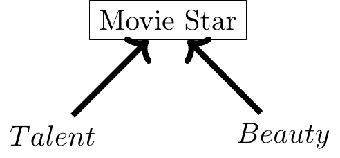
Let’s illustrate this with a simple program.

Stata Code

moviestar.do

clear all 
set seed 3444 

* 2500 independent draws from standard normal distribution 
set obs 2500 
generate beauty=rnormal() 
generate talent=rnormal() 

* Creating the collider variable (star) 
gen score=(beauty+talent) 
egen c85=pctile(score), p(85)   
gen star=(score>=c85) 
label variable star "Movie star" 

* Conditioning on the top 15\% 
twoway (scatter beauty talent, mcolor(black) msize(small) msymbol(smx)), ytitle(Beauty) xtitle(Talent) subtitle(Aspiring actors and actresses) by(star, total)

R Code

moviestar.R

library(tidyverse)
library(patchwork)

set.seed(3444)

star_is_born <- tibble(
  beauty = rnorm(2500),
  talent = rnorm(2500),
  score = beauty + talent,
  c85 = quantile(score, .85),
  star = ifelse(score>=c85,1,0)
)

p1 = star_is_born %>% 
  ggplot(aes(x = talent, y = beauty)) +
  geom_point(size = 1, alpha = 0.5) + xlim(-4, 4) + ylim(-4, 4) + 
  geom_smooth(method = 'lm', se = FALSE) + 
  labs(title = "Everyone")

p2 = star_is_born %>% 
  ggplot(aes(x = talent, y = beauty, color = factor(star))) +
  geom_point(size = 1, alpha = 0.25) + xlim(-4, 4) + ylim(-4, 4) + 
  geom_smooth(method = 'lm', se = FALSE) + 
  labs(title = "Everyone, but different") +
  scale_color_discrete(name = 'Star')

p1 + p2

Python Code

moviestar.py

import numpy as np 
import pandas as pd 
import statsmodels.api as sm 
import statsmodels.formula.api as smf 
from itertools import combinations 
import plotnine as p
from stargazer.stargazer import Stargazer

# read data
import ssl
ssl._create_default_https_context = ssl._create_unverified_context
def read_data(file): 
    return pd.read_stata("https://github.com/scunning1975/mixtape/raw/master/" + file)



start_is_born = pd.DataFrame({
    'beauty': np.random.normal(size=2500),
    'talent': np.random.normal(size=2500)})
    
start_is_born['score'] = start_is_born['beauty'] + start_is_born['talent']
start_is_born['c85'] = np.percentile(start_is_born['score'], q=85)
start_is_born['star'] = 0
start_is_born.loc[start_is_born['score']>start_is_born['c85'], 'star'] = 1
start_is_born.head()


lm = sm.OLS.from_formula('beauty ~ talent', data=start_is_born).fit()

p.ggplot(start_is_born, p.aes(x='talent', y='beauty')) +    p.geom_point(size = 0.5) +    p.xlim(-4, 4) +    p.ylim(-4, 4)

p.ggplot(start_is_born[start_is_born.star==1], p.aes(x='talent', y='beauty')) +    p.geom_point(size = 0.5) +    p.xlim(-4, 4) +    p.ylim(-4, 4)

p.ggplot(start_is_born[start_is_born.star==0], p.aes(x='talent', y='beauty')) +    p.geom_point(size = 0.5) +    p.xlim(-4, 4) +    p.ylim(-4, 4)

Figure 3.1 shows the output from this simulation. The bottom left panel shows the scatter plot between talent and beauty. Notice that the two variables are independent, random draws from the standard normal distribution, creating an oblong data cloud. But because “movie star” is in the top 85th percentile of the distribution of a linear combination of talent and beauty, the sample consists of people whose combined score is in the top right portion of the joint distribution. This frontier has a negative slope and is in the upper right portion of the data cloud, creating a negative correlation between the observations in the movie-star sample. Likewise, the collider bias has created a negative correlation between talent and beauty in the non-movie-star sample as well. Yet we know that there is in fact no relationship between the two variables. This kind of sample selection creates spurious correlations. A random sample of the full population would be sufficient to show that there is no relationship between the two variables, but splitting the sample into movie stars only, we introduce spurious correlations between the two variables of interest.

Figure 3.1: Top left figure: Non-star sample scatter plot of beauty (vertical axis) and talent (horizontal axis). Top right right figure: Star sample scatter plot of beauty and talent. Bottom left figure: Entire (stars and non-stars combined) sample scatter plot of beauty and talent.

3.1.7 Collider bias and police use of force

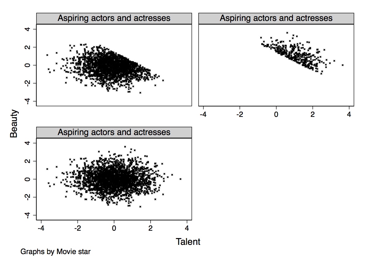
We’ve known about the problems of nonrandom sample selection for decades (J. J. Heckman 1979). But DAGs may still be useful for helping spot what might be otherwise subtle cases of conditioning on colliders (Elwert and Winship 2014). And given the ubiquitous rise in researcher access to large administrative databases, it’s also likely that some sort of theoretically guided reasoning will be needed to help us determine whether the databases we have are themselves rife with collider bias. A contemporary debate could help illustrate what I mean.

Public concern about police officers systematically discriminating against minorities has reached a breaking point and led to the emergence of the Black Lives Matter movement. “Vigilante justice” episodes such as George Zimmerman’s killing of teenage Trayvon Martin, as well as police killings of Michael Brown, Eric Garner, and countless others, served as catalysts to bring awareness to the perception that African Americans face enhanced risks for shootings. Fryer (2019) attempted to ascertain the degree to which there was racial bias in the use of force by police. This is perhaps one of the most important questions in policing as of this book’s publication.

There are several critical empirical challenges in studying racial biases in police use of force, though. The main problem is that all data on police-citizen interactions are conditional on an interaction having already occurred. The data themselves were generated as a function of earlier police-citizen interactions. In this sense, we can say that the data itself are endogenous. Fryer (2019) collected several databases that he hoped would help us better understand these patterns. Two were public-use data sets—the New York City Stop and Frisk database and the Police-Public Contact Survey. The former was from the New York Police Department and contained data on police stops and questioning of pedestrians; if the police wanted to, they could frisk them for weapons or contraband. The latter was a survey of civilians describing interactions with the police, including the use of force.

But two of the data sets were administrative. The first was a compilation of event summaries from more than a dozen large cities and large counties across the United States from all incidents in which an officer discharged a weapon at a civilian. The second was a random sample of police-civilian interactions from the Houston Police Department. The accumulation of these databases was by all evidence a gigantic empirical task. For instance, Fryer (2019) notes that the Houston data was based on arrest narratives that ranged from two to one hundred pages in length. From these arrest narratives, a team of researchers collected almost three hundred variables relevant to the police use of force on the incident. This is the world in which we now live, though. Administrative databases can be accessed more easily than ever, and they are helping break open the black box of many opaque social processes.

A few facts are important to note. First, using the stop-and-frisk data, Fryer finds that blacks and Hispanics were more than 50 percent more likely to have an interaction with the police in the raw data. The racial difference survives conditioning on 125 baseline characteristics, encounter characteristics, civilian behavior, precinct, and year fixed effects. In his full model, blacks are 21 percent more likely than whites to be involved in an interaction with police in which a weapon is drawn (which is statistically significant). These racial differences show up in the Police-Public Contact Survey as well, only here the racial differences are considerably larger. So the first thing to note is that the actual stop itself appears to be larger for minorities, which I will come back to momentarily.

Things become surprising when Fryer moves to his rich administrative data sources. He finds that conditional on a police interaction, there are no racial differences in officer-involved shootings. In fact, controlling for suspect demographics, officer demographics, encounter characteristics, suspect weapon, and year fixed effects, blacks are 27 percent less likely to be shot at by police than are nonblack non-Hispanics. The coefficient is not significant, and it shows up across alternative specifications and cuts of the data. Fryer is simply unable with these data to find evidence for racial discrimination in officer-involved shootings.

One of the main strengths of Fryer’s study are the shoe leather he used to accumulate the needed data sources. Without data, one cannot study the question of whether police shoot minorities more than they shoot whites. And the extensive coding of information from the narratives is also a strength, for it afforded Fryer the ability to control for observable confounders. But the study is not without issues that could cause a skeptic to take issue. Perhaps the police departments most willing to cooperate with a study of this kind are the ones with the least racial bias, for instance. In other words, maybe these are not the departments with the racial bias to begin with.⁹ Or perhaps a more sinister explanation exists, such as records being unreliable because administrators scrub out the data on racially motivated shootings before handing them over to Fryer altogether.

But I would like to discuss a more innocent possibility, one that requires no conspiracy theories and yet is so basic a problem that it is in fact more worrisome. Perhaps the administrative datasource is endogenous because of conditioning on a collider. If so, then the administrative data itself may have the racial bias baked into it from the start. Let me explain with a DAG.

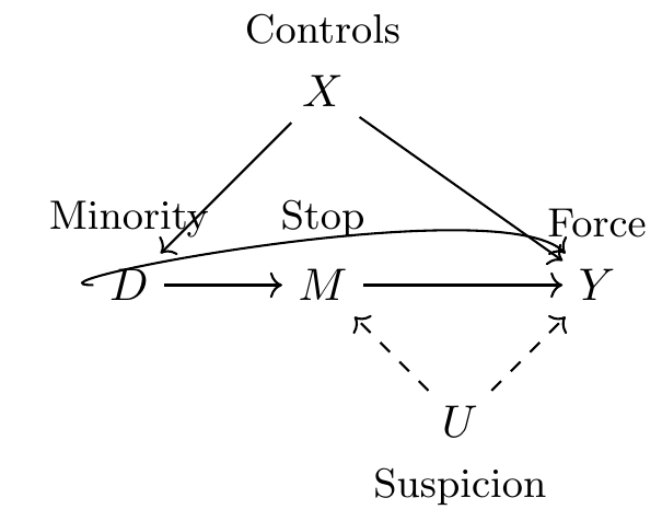
Fryer showed that minorities were more likely to be stopped using both the stop-and-frisk data and the Police-Public Contact Survey. So we know already that the \(D \rightarrow M\) pathway exists. In fact, it was a very robust correlation across multiple studies. Minorities are more likely to have an encounter with the police. Fryer’s study introduces extensive controls about the nature of the interaction, time of day, and hundreds of factors that I’ve captured with \(X\). Controlling for \(X\) allows Fryer to shut this backdoor path.

But notice \(M\)—the stop itself. All the administrative data is conditional on a stop. Fryer (2019) acknowledges this from the outset: “Unless otherwise noted, all results are conditional on an interaction. Understanding potential selection into police data sets due to bias in who police interacts with is a difficult endeavor” (3). Yet what this DAG shows is that if police stop people who they believe are suspicious and use force against people they find suspicious, then conditioning on the stop is equivalent to conditioning on a collider. It opens up the \(D \rightarrow M \leftarrow U \rightarrow Y\) mediated path, which introduces spurious patterns into the data that, depending on the signs of these causal associations, may distort any true relationship between police and racial differences in shootings.

Dean Knox, Will Lowe, and Jonathan Mummolo are a talented team of political scientists who study policing, among other things. They produced a study that revisited Fryer’s question and in my opinion both yielded new clues as to the role of racial bias in police use of force and the challenges of using administrative data sources to do so. I consider Knox, Lowe, and Mummolo (2020) one of the more methodologically helpful studies for understanding this problem and attempting to solve it. The study should be widely read by every applied researcher whose day job involves working with proprietary administrative data sets, because this DAG may in fact be a more general problem. After all, administrative data sources are already select samples, and depending on the study question, they may constitute a collider problem of the sort described in this DAG. The authors develop a bias correction procedure that places bounds on the severity of the selection problems. When using this bounding approach, they find that even lower-bound estimates of the incidence of police violence against civilians is as much as five times higher than a traditional approach that ignores the sample selection problem altogether.

It is incorrect to say that sample selection problems were unknown without DAGs. We’ve known about them and have had some limited solutions to them since at least J. J. Heckman (1979). What I have tried to show here is more general. An atheoretical approach to empiricism will simply fail. Not even “big data” will solve it. Causal inference is not solved with more data, as I argue in the next chapter. Causal inference requires knowledge about the behavioral processes that structure equilibria in the world. Without them, one cannot hope to devise a credible identification strategy. Not even data is a substitute for deep institutional knowledge about the phenomenon you’re studying. That, strangely enough, even includes the behavioral processes that generated the samples you’re using in the first place. You simply must take seriously the behavioral theory that is behind the phenomenon you’re studying if you hope to obtain believable estimates of causal effects. And DAGs are a helpful tool for wrapping your head around and expressing those problems.

3.2 Conclusion

In conclusion, DAGs are powerful tools.¹⁰ They are helpful at both clarifying the relationships between variables and guiding you in a research design that has a shot at identifying a causal effect. The two concepts we discussed in this chapter—the backdoor criterion and collider bias—are but two things I wanted to bring to your attention. And since DAGs are themselves based on counterfactual forms of reasoning, they fit well with the potential outcomes model that I discuss in the next chapter.

Causal Inference:
The Mixtape.

Buy the print version today:

Buy from Amazon Buy from Yale Press

Angrist, Joshua D., and Jorn-Steffen Pischke. 2009. Mostly Harmless Econometrics. 1st ed. Princeton University Press.

Becker, Gary. 1994. Human Capital: A Theoretical and Empirical Analysis with Special Reference to Education. 3rd ed. University of Chicago Press.

Elwert, Felix, and Christopher Winship. 2014. “Endogenous Selection Bias: The Problem of Conditioning on a Collider Variable.” Annual Review of Sociology 40: 31–53.

Fryer, Roland. 2019. “An Empirical Analysis of Racial Differences in Police Use of Force.” Journal of Political Economy 127 (3).

Heckman, James J. 1979. “Sample Selection Bias as a Specificaiton Error.” Econometrica 47 (1): 153–61.

Heckman, James, and Rodrigo Pinto. 2015. “Causal Analysis After Haavelmo.” Econometric Theory 31 (1): 115–51.

Imbens, Guido W. 2019. “Potential Outcome and Directed Acyclic Graph Approaches to Causality: Relevance for Empirical Practices in Economics.”

Knox, Dean, Will Lowe, and Jonathan Mummolo. 2020. “Administrative Records Mask Racially Biased Policing.” American Political Science Review Forthcoming.

Matsueda, Ross L. 2012. “Handbook of Structural Equation Modeling.” In. Guilford Press.

Morgan, Stephen L., and Christopher Winship. 2014. Counterfactuals and Causal Inference: Methods and Principles for Social Research. 2nd ed. Cambridge University Press.

Pearl, Judea. 2009. Causality. 2nd ed. Cambridge University Press.

Piazza, Jo. 2009. “Megan Fox Voted Worst - but Sexiest - Actress of 2009.” https://marquee.blogs.cnn.com/2009/12/30/megan-fox-voted-worst-but-sexiest-actress-of-2009/.

Wolpin, Kenneth I. 2013. The Limits of Inference Without Theory. MIT Press.

---

1. I will discuss the Wrights again in the chapter on instrumental variables. They were an interesting pair.

2. If you find this material interesting, I highly recommend Morgan and Winship (2014), an all-around excellent book on causal inference, and especially on graphical models.

3. I leave out some of those details, though, because their presence (usually just error terms pointing to the variables) clutters the graph unnecessarily.

4. Subsequent chapters discuss other estimators, such as matching.

5. Productivity could diverge, though, if women systematically sort into lower-quality occupations in which human capital accumulates over time at a lower rate.

6. Angrist and Pischke (2009) talk about this problem in a different way using language called “bad controls.” Bad controls are not merely conditioning on outcomes. Rather, they are any situation in which the outcome had been a collider linking the treatment to the outcome of interest, like \(D\) \(\rightarrow O \leftarrow A \rightarrow Y\).

7. Erin Hengel is a professor of economics at the University of Liverpool. She and I were talking about this on Twitter one day, and she and I wrote down the code describing this problem. Her code was better, so I asked if I could reproduce it here, and she said yes. Erin’s work partly focuses on gender discrimination. You can see some of that work on her website at http://www.erinhengel.com.

8. I wish I had thought of this example, but alas the sociologist Gabriel Rossman gets full credit.

9. I am not sympathetic to this claim. The administrative data comes from large Texas cities, a large county in California, the state of Florida, and several other cities and counties racial bias has been reported.

10. There is far more to DAGs than I have covered here. If you are interested in learning more about them, then I encourage you to carefully read Pearl (2009), which is his magnum opus and a major contribution to the theory of causation.