2 Probability and Regression Review

Causal Inference:
The Mixtape.

Buy the print version today:

\[ % Define terms \newcommand{\Card}{\text{Card }} \DeclareMathOperator*{\cov}{cov} \DeclareMathOperator*{\var}{var} \DeclareMathOperator{\Var}{Var\,} \DeclareMathOperator{\Cov}{Cov\,} \DeclareMathOperator{\Prob}{Prob} \DeclareMathOperator{\Pr}{Pr} \newcommand{\independent}{\perp \!\!\! \perp} \DeclareMathOperator{\Post}{Post} \DeclareMathOperator{\Pre}{Pre} \DeclareMathOperator{\Mid}{\,\vert\,} \DeclareMathOperator{\post}{post} \DeclareMathOperator{\pre}{pre} \]

2.1 Basic probability theory

In practice, causal inference is based on statistical models that range from the very simple to extremely advanced. And building such models requires some rudimentary knowledge of probability theory, so let’s begin with some definitions. A random process is a process that can be repeated many times with different outcomes each time. The sample space is the set of all the possible outcomes of a random process. We distinguish between discrete and continuous random processes Table 1 below. Discrete processes produce, integers, whereas continuous processes produce fractions as well.

Table 2.1: Examples of Discrete and Continuous Random Processes

Description	Type	Potential outcomes
12-sided die	Discrete	1, 2, 3, 4, 5, 6, 7, 8, 9, 10, 11, 12
Coin	Discrete	Heads, Tails
Deck of cards	Discrete	2 $\diamondsuit$, 3 $\diamondsuit$, …King $\heartsuit$, Ace $\heartsuit$
Gas prices	Continuous	$P\geq 0$

We define independent events two ways. The first refers to logical independence. For instance, two events occur but there is no reason to believe that the two events affect each other. When it is assumed that they do affect each other, this is a logical fallacy called post hoc ergo propter hoc, which is Latin for “after this, therefore because of this.” This fallacy recognizes that the temporal ordering of events is not sufficient to be able to say that the first thing caused the second.

The second definition of an independent event is statistical independence. We’ll illustrate the latter with an example from the idea of sampling with and without replacement. Let’s use a randomly shuffled deck of cards for an example. For a deck of 52 cards, what is the probability that the first card will be an ace? \[ \Pr(\text{Ace}) =\dfrac{\text{Count Aces}}{\text{Sample Space}}=\dfrac{4}{52}= \dfrac{1}{13}=0.077 \] There are 52 possible outcomes in the sample space, or the set of all possible outcomes of the random process. Of those 52 possible outcomes, we are concerned with the frequency of an ace occurring. There are four aces in the deck, so $\dfrac{4}{52}=0.077$.

Assume that the first card was an ace. Now we ask the question again. If we shuffle the deck, what is the probability the next card drawn is also an ace? It is no longer $\dfrac{1}{13}$ because we did not sample with replacement. We sampled without replacement. Thus the new probability is \[ \Pr\Big(\text{Ace}\mid\text{Card } 1 =\text{Ace}\Big) = \dfrac{3}{51}= 0.059 \] Under sampling without replacement, the two events—ace on $\text{Card } 1$ and an ace on $\text{Card } 2$ if $\text{Card } 1$ was an ace—aren’t independent events. To make the two events independent, you would have to put the ace back and shuffle the deck. So two events, $A$ and $B$, are independent if and only if: \[ \Pr(A\mid B)=\Pr(A) \] An example of two independent events would be rolling a 5 with one die after having rolled a 3 with another die. The two events are independent, so the probability of rolling a 5 is always 0.17 regardless of what we rolled on the first die.¹

But what if we want to know the probability of some event occurring that requires that multiple events first to occur? For instance, let’s say we’re talking about the Cleveland Cavaliers winning the NBA championship. In 2016, the Golden State Warriors were 3–1 in a best-of-seven playoff. What had to happen for the Warriors to lose the playoff? The Cavaliers had to win three in a row. In this instance, to find the probability, we have to take the product of all marginal probabilities, or $\Pr(\cdot)^n$, where $\Pr(\cdot)$ is the marginal probability of one event occurring, and $n$ is the number of repetitions of that one event. If the unconditional probability of a Cleveland win is 0.5, and each game is independent, then the probability that Cleveland could come back from a 3–1 deficit is the product of each game’s probability of winning: \[ \text{Win probability} =\Pr\big(W,W,W\big)= (0.5)^3= 0.125 \] Another example may be helpful. In Texas Hold’em poker, each player is dealt two cards facedown. When you are holding two of a kind, you say you have two “in the pocket.” So, what is the probability of being dealt pocket aces? It’s $\dfrac{4}{52}\times\dfrac{3}{51}=0.0045$. That’s right: it’s $0.45\%$.

Let’s formalize what we’ve been saying for a more generalized case. For independent events, to calculate joint probabilities, we multiply the marginal probabilities: \[ \Pr(A,B)=\Pr(A)\Pr(B) \] where $\Pr(A,B)$ is the joint probability of both $A$ and $B$ occurring, and $\Pr(A)$ is the marginal probability of $A$ event occurring.

Now, for a slightly more difficult application. What is the probability of rolling a 7 using two six-sided dice, and is it the same as the probability of rolling a 3? To answer this, let’s compare the two probabilities. We’ll use a table to help explain the intuition. First, let’s look at all the ways to get a 7 using two six-sided dice. There are 36 total possible outcomes $(6^2=36)$ when rolling two dice. In Table 2.2 we see that there are six different ways to roll a 7 using only two dice. So the probability of rolling a 7 is $6/36=16.67$%. Next, let’s look at all the ways to roll a 3 using two six-sided dice. Table 2.3 shows that there are only two ways to get a 3 rolling two six-sided dice. So the probability of rolling a 3 is $2/36=5.56$%. So, no, the probabilities of rolling a 7 and rolling a 3 are different.

Table 2.2: Total number of ways to get a 7 with two six-sided dice.

Die 1	Die 2	Outcome
1	6	7
2	5	7
3	4	7
4	3	7
5	2	7
6	1	7

Table 2.3: Total number of ways to get a 3 using two six-sided dice.

Die 1	Die 2	Outcome
1	2	3
2	1	3

2.2 Events and conditional probability

First, before we talk about the three ways of representing a probability, I’d like to introduce some new terminology and concepts: events and conditional probabilities. Let $A$ be some event. And let $B$ be some other event. For two events, there are four possibilities.

A and B: Both A and B occur.
$\sim$ A and B: A does not occur, but B occurs.
A and $\sim$ B: A occurs, but B does not occur.
$\sim$ A and $\sim$ B: Neither A nor B occurs.

I’ll use a couple of different examples to illustrate how to represent a probability.

2.3 Probability tree

Let’s think about a situation in which you are trying to get your driver’s license. Suppose that in order to get a driver’s license, you have to pass the written exam and the driving exam. However, if you fail the written exam, you’re not allowed to take the driving exam. We can represent these two events in a probability tree.

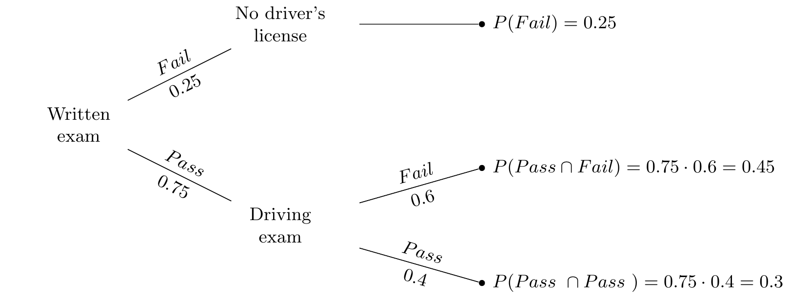
Probability trees are intuitive and easy to interpret.² First, we see that the probability of passing the written exam is 0.75 and the probability of failing the exam is 0.25. Second, at every branching off from a node, we can further see that the probabilities associated with a given branch are summing to 1.0. The joint probabilities are also all summing to 1.0. This is called the law of total probability and it is equal to the sum of all joint probability of A and B$_n$ events occurring: \[ \Pr(A)=\sum_n Pr(A\cap B_n) \]

We also see the concept of a conditional probability in the driver’s license tree. For instance, the probability of failing the driving exam, conditional on having passed the written exam, is represented as $\Pr(\text{Fail} \mid \text{Pass})= 0.45/0.75 = 0.6$.

2.4 Venn diagrams and sets

A second way to represent multiple events occurring is with a Venn diagram. Venn diagrams were first conceived by John Venn in 1880. They are used to teach elementary set theory, as well as to express set relationships in probability and statistics. This example will involve two sets, $A$ and $B$.

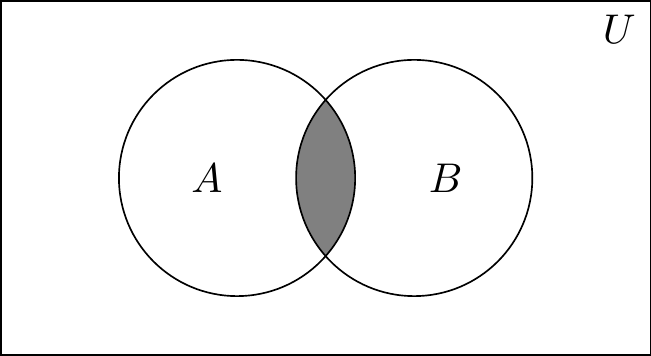
The University of Texas’s football coach has been on the razor’s edge with the athletic director and regents all season. After several mediocre seasons, his future with the school is in jeopardy. If the Longhorns don’t make it to a great bowl game, he likely won’t be rehired. But if they do, then he likely will be rehired. Let’s discuss elementary set theory using this coach’s situation as our guiding example. But before we do, let’s remind ourselves of our terms. $A$ and $B$ are events, and $U$ is the universal set of which $A$ and $B$ are subsets. Let $A$ be the probability that the Longhorns get invited to a great bowl game and $B$ be the probability that their coach is rehired. Let $\Pr(A)=0.6$ and let $\Pr(B)=0.8$. Let the probability that both $A$ and $B$ occur be $\Pr(A,B)=0.5$.

Note, that $A+\sim A=U$, where $\sim A$ is the complement of $A$. The complement means that it is everything in the universal set that is not A. The same is said of B. The sum of $B$ and $\sim B=U$. Therefore: \[ A+{\sim} A=B+ {\sim} B \]

We can rewrite out the following definitions:

\[\begin{align} A & = B+{\sim} B - {\sim} A \\ B & = A+{\sim} A - {\sim} B \end{align}\]

Whenever we want to describe a set of events in which either $A$ or $B$ could occur, it is: $A \cup B$. And this is pronounced “$A$ union $B$,” which means it is the new set that contains every element from $A$ and every element from $B$. Any element that is in either set $A$ or set $B$, then, is also in the new union set. And whenever we want to describe a set of events that occurred together—the joint set—it’s $A \cap B$, which is pronounced “$A$ intersect $B$.” This new set contains every element that is in both the $A$ and $B$ sets. That is, only things inside both $A$ and $B$ get added to the new set.

Now let’s look closely at a relationship involving the set A.

\[\begin{align} A=A \cap B+A \cap{\sim} B \end{align}\]

Notice what this is saying: there are two ways to identify the $A$ set. First, you can look at all the instances where $A$ occurs with $B$. But then what about the rest of $A$ that is not in $B$? Well, that’s the $A \cap \sim B$ situation, which covers the rest of the $A$ set.

A similar style of reasoning can help you understand the following expression. \[ A \cup B=A \cap{\sim}B+\sim A \cap B+A \cap B \] To get $A$ union $B$, we need three objects: the set of $A$ units outside of $B$, the set of $B$ units outside $A$, and their joint set. To get $A \cup B$, just rearrange the previous equation.

Now it is just simple addition to find all missing values. Recall that $A$ is your team making playoffs and $\Pr(A)=0.6$. And $B$ is the probability that the coach is rehired, $\Pr(B)=0.8$. Also, $\Pr(A,B)=0.5$, which is the probability of both $A$ and $B$ occurring. Then we have:

\[\begin{align} A & = A \cap B+A \cap{\sim}B \\ A \cap{\sim}B & = A - A \cap B \\ \Pr(A, \sim B) & = \Pr(A) - Pr(A,B) \\ \Pr(A,\sim B) & = 0.6 - 0.5 \\ \Pr(A,\sim B) & = 0.1 \end{align}\]

When working with sets, it is important to understand that probability is calculated by considering the share of the set (for example $A$) made up by the subset (for example $A \cap B$). When we write down that the probability that $A \cap B$ occurs at all, it is with regards to $U$. But what if we were to ask the question “What share of A is due to $A \cap B$?” Notice, then, that we would need to do this:

\[\begin{align} ? & = A \cap B \div A \\ ? & = 0.5 \div 0.6 \\ ? & = 0.83 \end{align}\]

I left this intentionally undefined on the left side so as to focus on the calculation itself. But now let’s define what we are wanting to calculate: In a world where $A$ has occurred, what is the probability that $B$ will also occur? This is:

\[\begin{align} \Pr(B \mid A) & = \dfrac{\Pr(A,B)}{\Pr(A)}= \dfrac{0.5}{0.6}=0.83 \\ \Pr(A \mid B) & = \dfrac{\Pr(A,B)}{\Pr(B)}= \dfrac{0.5}{0.8}=0.63 \end{align}\] Notice, these conditional probabilities are not as easy to see in the Venn diagram. We are essentially asking what percentage of a subset—e.g., $\Pr(A)$—is due to the joint set, for example, $\Pr(A,B)$. This reasoning is the very same reasoning used to define the concept of a conditional probability.

2.5 Contingency tables

Another way that we can represent events is with a contingency table. Contingency tables are also sometimes called twoway tables. Table 2.4 is an example of a contingency table. We continue with our example about the worried Texas coach.

Table 2.4: Two way contingency table.

Event labels	Coach is not rehired $(\sim B)$	Coach is rehired $(B)$	Total
$(A)$ Bowl game	$\Pr(A,\sim B)$=0.1	$\Pr(A,B)$=0.5	$\Pr(A)$=0.6
$(\sim A)$ no Bowl game	$\Pr(\sim A, \sim B)=0.1$	$\Pr(\sim A,B)=0.3$	$\Pr(\sim A)=0.4$
Total	$\Pr(\sim B)=0.2$	$\Pr(B)=0.8$	1.0

Recall that $\Pr(A)=0.6$, $\Pr(B)=0.8$, and $Pr(A,B)=0.5$. Note that to calculate conditional probabilities, we must know the frequency of the element in question (e.g., $\Pr(A,B)$) relative to some other larger event (e.g., $\Pr(A)$). So if we want to know what the conditional probability of $B$ is given $A$, then it’s: \[ \Pr(B\mid A)=\dfrac{\Pr(A,B)}{\Pr(A)}=\dfrac{0.5}{0.6}=0.83 \] But note that knowing the frequency of $A\cap B$ in a world where $B$ occurs is to ask the following: \[ \Pr(A\mid B)=\dfrac{\Pr(A,B)}{\Pr(B)}= \dfrac{0.5}{0.8}=0.63 \]

So, we can use what we have done so far to write out a definition of joint probability. Let’s start with a definition of conditional probability first. Given two events, $A$ and $B$: \[\begin{align} \Pr(A\mid B) &= \frac{\Pr(A,B)}{\Pr(B)} \\ \Pr(B\mid A) &= \frac{\Pr(B,A)}{\Pr(A)} \\ \Pr(A,B) &= \Pr(B,A) \\ \Pr(A) &= \Pr(A,\sim B)+\Pr(A,B) \\ \Pr(B) &= \Pr(A,B)+\Pr(\sim A, B) \end{align}\]

Using equations (1) and (2), I can simply write down a definition of joint probabilities.

\[ \Pr(A,B) = \Pr(A \mid B) \Pr(B) \tag{2.1}\]

\[ \Pr(B,A) = \Pr(B \mid A) \Pr(A) \tag{2.2}\]

And this is the formula for joint probability. Given equation (3), and using the definitions of $(\Pr(A,B)$ and $\Pr(B,A))$, I can also rearrange terms, make a substitution, and rewrite it as:

\[ \Pr(A\mid B)\Pr(B) = \Pr(B\mid A)\Pr(A) \]

\[ \Pr(A\mid B) = \frac{\Pr(B\mid A) \Pr(A)}{\Pr(B)} \tag{2.3}\]

Equation 2.3 is sometimes called the naive version of Bayes’s rule. We will now decompose this equation more fully, though, by substituting equation (5) into Equation 2.3.

\[ \Pr(A\mid B) = \frac{\Pr(B\mid A)\Pr(A)}{\Pr(A,B) + \Pr(\sim A,B)} \tag{2.4}\]

Substituting Equation 2.1 into the denominator for Equation 2.4 yields:

\[ \Pr(A\mid B)=\frac{\Pr(B\mid A)\Pr(A)}{\Pr(B\mid A)\Pr(A)+\Pr(\sim A, B)} \tag{2.5}\] Finally, we note that using the definition of joint probability, that $\Pr(B,\sim A)= \Pr(B\mid\sim A)\Pr(\sim A)$, which we substitute into the denominator of Equation 2.5 to get:

\[ \Pr(A\mid B)=\frac{\Pr(B\mid A)\Pr(A)}{\Pr(B\mid A)\Pr(A)+\Pr(B\mid \sim A)\Pr(\sim A)} \tag{2.6}\]

That’s a mouthful of substitutions, so what does Equation 2.6 mean? This is the Bayesian decomposition version of Bayes’s rule. Let’s use our example again of Texas making a great bowl game. $A$ is Texas making a great bowl game, and $B$ is the coach getting rehired. And $A\cup B$ is the joint probability that both events occur. We can make each calculation using the contingency tables. The questions here is this: If the Texas coach is rehired, what’s the probability that the Longhorns made a great bowl game? Or formally, $\Pr(A\mid B)$. We can use the Bayesian decomposition to find this probability.

\[\begin{align} \Pr(A\mid B) & = \dfrac{\Pr(B\mid A)\Pr(A)}{\Pr(B\mid A)\Pr(A)+\Pr(B\mid \sim A)\Pr(\sim A)} \\ & =\dfrac{0.83\cdot 0.6}{0.83\cdot 0.6+0.75\cdot 0.4} \\ & =\dfrac{0.498}{0.498+0.3} \\ & =\dfrac{0.498}{0.798} \\ \Pr(A\mid B) & =0.624 \end{align}\] Check this against the contingency table using the definition of joint probability:

\[\begin{align} \Pr(A\mid B)=\dfrac{\Pr(A,B)}{\Pr(B)}= \dfrac{0.5}{0.8}=0.625 \end{align}\] So, if the coach is rehired, there is a 63 percent chance we made a great bowl game.³

2.6 Monty Hall example

Let’s use a different example, the Monty Hall example. This is a fun one, because most people find itcounterintuitive. It even is used to stump mathematicians and statisticians.⁴ But Bayes’s rule makes the answer very clear—so clear, in fact, that it’s somewhat surprising that Bayes’s rule was actually once controversial (Mcgrayne 2012).

Let’s assume three closed doors: door 1 $(D_1)$, door 2 $(D_2)$, and door 3 $(D_3)$. Behind one of the doors is a million dollars. Behind each of the other two doors is a goat. Monty Hall, the game-show host in this example, asks the contestants to pick a door. After they pick the door, but before he opens the door they picked, he opens one of the other doors to reveal a goat. He then asks the contestant, “Would you like to switch doors?”

A common response to Monty Hall’s offer is to say it makes no sense to change doors, because there’s an equal chance that the million dollars is behind either door. Therefore, why switch? There’s a 50–50 chance it’s behind the door picked and there’s a 50–50 chance it’s behind the remaining door, so it makes no rational sense to switch. Right? Yet, a little intuition should tell you that’s not the right answer, because it would seem that when Monty Hall opened that third door, he made a statement. But what exactly did he say?

Let’s formalize the problem using our probability notation. Assume that you chose door 1, $D_1$. The probability that $D_1$ had a million dollars when you made that choice is $\Pr(D_1=1 \text{ million})=\dfrac{1}{3}$. We will call that event $A_1$. And the probability that $D_1$ has a million dollars at the start of the game is $\dfrac{1}{3}$ because the sample space is 3 doors, of which one has a million dollars behind it. Thus, $\Pr(A_1)=\dfrac{1}{3}$. Also, by the law of total probability, $\Pr(\sim A_1)=\dfrac{2}{3}$. Let’s say that Monty Hall had opened door 2, $D_2$, to reveal a goat. Then he asked, “Would you like to change to door number 3?”

We need to know the probability that door 3 has the million dollars and compare that to Door 1’s probability. We will call the opening of door 2 event $B$. We will call the probability that the million dollars is behind door $i$, $A_i$. We now write out the question just asked formally and decompose it using the Bayesian decomposition. We are ultimately interested in knowing what the probability is that door 1 has a million dollars (event $A_1$) given that Monty Hall opened door 2 (event $B$), which is a conditional probability question. Let’s write out that conditional probability using the Bayesian decomposition from Equation 2.6.

\[ \Pr(A_1 \mid B) = \dfrac{\Pr(B\mid A_1) \Pr(A_1)}{\Pr(B\mid A_1) \Pr(A_1)+\Pr(B\mid A_2) \Pr(A_2)+\Pr(B\mid A_3) \Pr(A_3)} \tag{2.7}\]

There are basically two kinds of probabilities on the right side of the equation. There’s the marginal probability that the million dollars is behind a given door, $\Pr(A_i)$. And there’s the conditional probability that Monty Hall would open door 2 given that the million dollars is behind door $A_i$, $\Pr(B\mid A_i)$.

The marginal probability that door $i$ has the million dollars behind it without our having any additional information is $\dfrac{1}{3}$. We call this the prior probability, or prior belief. It may also be called the unconditional probability.

The conditional probability, $\Pr(B|A_i)$, requires a little more careful thinking. Take the first conditional probability, $\Pr(B\mid A_1)$. If door 1 has the million dollars behind it, what’s the probability that Monty Hall would open door 2?

Let’s think about the second conditional probability: $\Pr(B\mid A_2)$. If the money is behind door 2, what’s the probability that Monty Hall would open door 2?

And then the last conditional probability, $\Pr(B\mid A_3)$. In a world where the money is behind door 3, what’s the probability Monty Hall will open door 2?

Each of these conditional probabilities requires thinking carefully about the feasibility of the events in question. Let’s examine the easiest question: $\Pr(B\mid A_2)$. If the money is behind door 2, how likely is it for Monty Hall to open that same door, door 2? Keep in mind: this is a game show. So that gives you some idea about how the game-show host will behave. Do you think Monty Hall would open a door that had the million dollars behind it? It makes no sense to think he’d ever open a door that actually had the money behind it—he will always open a door with a goat. So don’t you think he’s only opening doors with goats? Let’s see what happens if take that intuition to its logical extreme and conclude that Monty Hall never opens a door if it has a million dollars. He only opens a door if the door has a goat. Under that assumption, we can proceed to estimate $\Pr(A_1\mid B)$ by substituting values for $\Pr(B\mid A_i)$ and $\Pr(A_i)$ into the right side of Equation 2.7.

What then is $\Pr(B\mid A_1)$? That is, in a world where you have chosen door 1, and the money is behind door 1, what is the probability that he would open door 2? There are two doors he could open if the money is behind door 1—he could open either door 2 or door 3, as both have a goat behind them. So $\Pr(B\mid A_1)=0.5$.

What about the second conditional probability, $\Pr(B\mid A_2)$? If the money is behind door 2, what’s the probability he will open it? Under our assumption that he never opens the door if it has a million dollars, we know this probability is 0.0. And finally, what about the third probability, $\Pr(B\mid A_3)$? What is the probability he opens door 2 given that the money is behind door 3? Now consider this one carefully—the contestant has already chosen door 1, so he can’t open that one. And he can’t open door 3, because that has the money behind it. The only door, therefore, he could open is door 2. Thus, this probability is 1.0. Furthermore, all marginal probabilities, $\Pr(A_i)$, equal 1/3, allowing us to solve for the conditional probability on the left side through substitution, multiplication, and division.

\[\begin{align} \Pr(A_1\mid B) & = \dfrac{\dfrac{1}{2}\cdot \dfrac{1}{3}}{\dfrac{1}{2}\cdot \dfrac{1}{3}+0\cdot\dfrac{1}{3}+1.0 \cdot \dfrac{1}{3}} \\ & =\dfrac{\dfrac{1}{6}}{\dfrac{1}{6}+\dfrac{2}{6}} \\ & = \dfrac{1}{3} \end{align}\] Aha. Now isn’t that just a little bit surprising? The probability that the contestant chose the correct door is $\dfrac{1}{3}$, just as it was before Monty Hall opened door 2.

But what about the probability that door 3, the door you’re holding, has the million dollars? Have your beliefs about that likelihood changed now that door 2 has been removed from the equation? Let’s crank through our Bayesian decomposition and see whether we learned anything.

\[\begin{align} \Pr(A_3\mid B) & = \dfrac{ \Pr(B\mid A_3)\Pr(A_3) }{ \Pr(B\mid A_3)\Pr(A_3)+\Pr(B\mid A_2)\Pr(A_2)+ \Pr(B\mid A_1)\Pr(A_1) } \\ & = \dfrac{ 1.0 \cdot \dfrac{1}{3} }{ 1.0 \cdot \dfrac{1}{3}+0 \cdot \dfrac{1}{3}+\dfrac{1}{2} \cdot \dfrac{1}{3}} \\ & = \dfrac{2}{3} \end{align}\]

Interestingly, while your beliefs about the door you originally chose haven’t changed, your beliefs about the other door have changed. The prior probability, $\Pr(A_3)=\dfrac{1}{3}$, increased through a process called updating to a new probability of $\Pr(A_3\mid B)=\dfrac{2}{3}$. This new conditional probability is called the posterior probability, or posterior belief. And it simply means that having witnessed $B$, you learned information that allowed you to form a new belief about which door the money might be behind.

As was mentioned in footnote 14 regarding the controversy around vos Sant’s correct reasoning about the need to switch doors, deductions based on Bayes’s rule are often surprising even to smart people—probably because we lack coherent ways to correctly incorporate information into probabilities. Bayes’s rule shows us how to do that in a way that is logical and accurate. But besides being insightful, Bayes’s rule also opens the door for a different kind of reasoning about cause and effect. Whereas most of this book has to do with estimating effects from known causes, Bayes’s rule reminds us that we can form reasonable beliefs about causes from known effects.

2.7 Summation operator

The tools we use to reason about causality rest atop a bedrock of probabilities. We are often working with mathematical tools and concepts from statistics such as expectations and probabilities. One of the most common tools we will use in this book is the linear regression model, but before we can dive into that, we have to build out some simple notation.⁵ We’ll begin with the summation operator. The Greek letter $\Sigma$ (the capital Sigma) denotes the summation operator. Let $x_1, x_2, \ldots, x_n$ be a sequence of numbers. We can compactly write a sum of numbers using the summation operator as:

\[\begin{align} \sum_{i=1}^nx_i \equiv x_1+x_2+\ldots+x_n \end{align}\] The letter $i$ is called the index of summation. Other letters, such as $j$ or $k$, are sometimes used as indices of summation. The subscript variable simply represents a specific value of a random variable, $x$. The numbers 1 and $n$ are the lower limit and the upper limit, respectively, of the summation. The expression $\Sigma_{i=1}^nx_i$ can be stated in words as “sum the numbers $x_i$ for all values of $i$ from 1 to $n$.” An example can help clarify:

\[\begin{align} \sum_{i=6}^9 x_i= x_6+x_7+x_8+x_9 \end{align}\] The summation operator has three properties. The first property is called the constant rule. Formally, it is:

For any constant $c$ \[ \sum_{i=1}^n c = nc \] Let’s consider an example. Say that we are given: \[ \sum_{i=1}^3 5=(5+5+5) = 3 \cdot 5=15 \] A second property of the summation operator is: \[ \sum_{i=1}^n c x_i = c\sum_{i=1}^nx_i \] Again let’s use an example. Say we are given:

\[\begin{align} \sum_{i=1}^3 5x_i & =5x_1+5x_2+5x_3 \\ & =5 (x_1+x_2+x_3) \\ & =5\sum_{i=1}^3x_i \end{align}\] We can apply both of these properties to get the following third property:

\[\begin{align} \text{For any constant $a$ and $b$:}\quad \sum_{i=1}^n(ax_i+by_i) =a\sum_{i=1}^n x_i + b\sum_{j=1}^n y_i \end{align}\] Before leaving the summation operator, it is useful to also note things which are not properties of this operator. First, the summation of a ratio is not the ratio of the summations themselves.

\[\begin{align} \sum_i^n \dfrac{x_i}{y_i} \ne \dfrac{ \sum_{i=1}^n x_i}{\sum_{i=1}^ny_i} \end{align}\] Second, the summation of some squared variable is not equal to the squaring of its summation.

\[\begin{align} \sum_{i=1}^nx_i^2 \ne \bigg(\sum_{i=1}^nx_i \bigg)^2 \end{align}\]

We can use the summation indicator to make a number of calculations, some of which we will do repeatedly over the course of this book. For instance, we can use the summation operator to calculate the average: \[\begin{align} \overline{x} & = \dfrac{1}{n} \sum_{i=1}^n x_i \\ & =\dfrac{x_1+x_2+\dots+x_n}{n} \end{align}\] where $\overline{x}$ is the average (mean) of the random variable $x_i$. Another calculation we can make is a random variable’s deviations from its own mean. The sum of the deviations from the mean is always equal to 0: \[ \sum_{i=1}^n (x_i - \overline{x})=0 \] You can see this in Table 2.5.

Table 2.5: Sum of deviations equalling zero

$x$	$x-\overline{x}$
10	2
4	$-4$
13	5
5	$-3$
Mean=8	Sum=0

Consider a sequence of two numbers {$y_1, y_2, \ldots, y_n$} and {$x_1, x_2, \ldots, x_n$}. Now we can consider double summations over possible values of $x$’s and $y$’s. For example, consider the case where $n=m=2$. Then, $\sum_{i=1}^2\sum_{j=1}^2x_iy_j$ is equal to $x_1y_1+x_1y_2+x_2y_1+x_2y_2$. This is because

\[\begin{align} x_1y_1+x_1y_2+x_2y_1+x_2y_2 & = x_1(y_1+y_2)+x_2(y_1+y_2) \\ & = \sum_{i=1}^2x_i(y_1+y_2) \\ & = \sum_{i=1}^2x_i \bigg( \sum_{j=1}^2y_j \bigg) \\ & = \sum_{i=1}^2 \bigg( \sum_{j=1}^2x_iy_j \bigg) \\ & = \sum_{i=1}^2 \sum_{j=1}^2x_iy_j \end{align}\] One result that will be very useful throughout the book is:

\[ \sum_{i=1}^n(x_i - \overline{x})^2=\sum_{i=1}^n x_i^2 - n(\overline{x})^2 \tag{2.8}\]

An overly long, step-by-step proof is below. Note that the summation index is suppressed after the first line for easier reading.

\[\begin{align} \sum_{i=1}^n(x_i-\overline{x})^2 & = \sum_{i=1}^n (x_i^2-2x_i\overline{x}+\overline{x}^2) \\ & = \sum x_i^2 - 2\overline{x} \sum x_i +n\overline{x}^2 \\ & = \sum x_i^2 - 2 \dfrac{1}{n} \sum x_i \sum x_i +n\overline{x}^2 \\ & = \sum x_i^2 +n\overline{x}^2 - \dfrac{2}{n} \bigg (\sum x_i \bigg )^2 \\ & = \sum x_i^2+n\bigg (\dfrac{1}{n} \sum x_i \bigg)^2 - 2n \bigg (\dfrac{1}{n} \sum x_i \bigg )^2 \\ & = \sum x_i^2 - n \bigg (\dfrac{1}{n} \sum x_i \bigg )^2 \\ & = \sum x_i^2 - n \overline{x}^2 \end{align}\]

A more general version of this result is:

\[\begin{align} \sum_{i=1}^n(x_i-\overline{x})(y_i-\overline{y}) & = \sum_{i=1}^n x_i(y_i - \overline{y}) \\ & = \sum_{i=1}^n (x_i - \overline{x})y_i \\ & = \sum_{i=1}^n x_iy_i - n(\overline{xy}) \\ \end{align}\]

Or: \[\begin{align} \sum_{i=1}^n (x_i -\overline{x})(y_i - \overline{y}) &= \sum_{i=1}^n x_i(y_i - \overline{y}) \\ &= \sum_{i=1}^n (x_i - \overline{x})y_i = \sum_{i=1}^n x_i y_i - n(\overline{x}\overline{y}) \end{align}\]

2.8 Expected value

The expected value of a random variable, also called the expectation and sometimes the population mean, is simply the weighted average of the possible values that the variable can take, with the weights being given by the probability of each value occurring in the population. Suppose that the variable $X$ can take on values $x_1, x_2, \ldots, x_k$, each with probability $f(x_1), f(x_2), \ldots, f(x_k)$, respectively. Then we define the expected value of $X$ as: \[\begin{align} E(X) & = x_1f(x_1)+x_2f(x_2)+\dots+x_kf(x_k) \\ & = \sum_{j=1}^k x_jf(x_j) \end{align}\] Let’s look at a numerical example. If $X$ takes on values of $-1$, 0, and 2, with probabilities 0.3, 0.3, and 0.4, respectively.⁶ Then the expected value of $X$ equals:

\[\begin{align} E(X) & = (-1)(0.3)+(0)(0.3)+(2)(0.4) \\ & = 0.5 \end{align}\] In fact, you could take the expectation of a function of that variable, too, such as $X^2$. Note that $X^2$ takes only the values 1, 0, and 4, with probabilities 0.3, 0.3, and 0.4. Calculating the expected value of $X^2$ therefore is:

\[\begin{align} E(X^2) & = (-1)^2(0.3)+(0)^2(0.3)+(2)^2(0.4) \\ & = 1.9 \end{align}\]

The first property of expected value is that for any constant $c$, $E(c)=c$. The second property is that for any two constants $a$ and $b$, then $E(aX+ b)=E(aX)+E(b)=aE(X)+b$. And the third property is that if we have numerous constants, $a_1, \dots, a_n$ and many random variables, $X_1, \dots, X_n$, then the following is true:

\[\begin{align} E(a_1X_1+\dots+a_nX_n)=a_1E(X_1)+\dots+a_nE(X_n) \end{align}\]

We can also express this using the expectation operator:

\[\begin{align} E\bigg(\sum_{i=1}^na_iX_i\bigg)=\sum_{i=1}a_iE(X_i) \end{align}\]

And in the special case where $a_i=1$, then

\[\begin{align} E\bigg(\sum_{i=1}^nX_i\bigg)=\sum_{i=1}^nE(X_i) \end{align}\]

2.9 Variance

The expectation operator, $E(\cdot)$, is a population concept. It refers to the whole group of interest, not just to the sample available to us. Its meaning is somewhat similar to that of the average of a random variable in the population. Some additional properties for the expectation operator can be explained assuming two random variables, $W$ and $H$.

\[\begin{align} E(aW+b) & = aE(W)+b\ \text{for any constants $a$, $b$} \\ E(W+H) & = E(W)+E(H) \\ E\Big(W - E(W)\Big) & = 0 \end{align}\] Consider the variance of a random variable, $W$:

\[\begin{align} V(W)=\sigma^2=E\Big[\big(W-E(W)\big)^2\Big]\ \text{in the population} \end{align}\] We can show \[ V(W)=E(W^2) - E(W)^2 \tag{2.9}\] In a given sample of data, we can estimate the variance by the following calculation:

\[\begin{align} \widehat{S}^2=(n-1)^{-1}\sum_{i=1}^n(x_i - \overline{x})^2 \end{align}\] where we divide by $n\ -\ 1$ because we are making a degree-of-freedom adjustment from estimating the mean. But in large samples, this degree-of-freedom adjustment has no practical effect on the value of $S^2$ where $S^2$ is the average (after a degree of freedom correction) over the sum of all squared deviations from the mean.⁷

A few more properties of variance. First, the variance of a line is: \[ V(aX+b)=a^2V(X) \tag{2.10}\]

And the variance of a constant is 0 (i.e., $V(c)=0$ for any constant, $c$). The variance of the sum of two random variables is equal to: \[ V(X+Y)=V(X)+V(Y)+2\Big(E(XY) - E(X)E(Y)\Big) \tag{2.11}\] If the two variables are independent, then $E(XY)=E(X)E(Y)$ and $V(X+Y)$ is equal to the sum of $V(X)+V(Y)$.

2.10 Covariance

The last part of Equation 2.11 is called the covariance. The covariance measures the amount of linear dependence between two random variables. We represent it with the $C(X,Y)$ operator. The expression $C(X,Y)>0$ indicates that two variables move in the same direction, whereas $C(X,Y)<0$ indicates that they move in opposite directions. Thus we can rewrite Equation 2.11 as:

\[\begin{align} V(X+Y)=V(X)+V(Y)+2C(X,Y) \end{align}\] While it’s tempting to say that a zero covariance means that two random variables are unrelated, that is incorrect. They could have a nonlinear relationship. The definition of covariance is \[ C(X,Y) = E(XY) - E(X)E(Y) \tag{2.12}\] As we said, if $X$ and $Y$ are independent, then $C(X,Y)=0$ in the population. The covariance between two linear functions is:

\[\begin{align} C(a_1+b_1X, a_2+b_2Y)=b_1b_2C(X,Y) \end{align}\] The two constants, $a_1$ and $a_2$, zero out because their mean is themselves and so the difference equals 0.

Interpreting the magnitude of the covariance can be tricky. For that, we are better served by looking at correlation. We define correlation as follows. Let $W=\dfrac{X-E(X)}{\sqrt{V(X)}}$ and $Z=\dfrac{Y - E(Y)}{\sqrt{V(Y)}}$. Then: \[ \text{Corr}(X,Y) = \text{Cov}(W,Z)=\dfrac{C(X,Y)}{\sqrt{V(X)V(Y)}} \tag{2.13}\] The correlation coefficient is bounded by $-1$ and 1. A positive (negative) correlation indicates that the variables move in the same (opposite) ways. The closer the coefficient is to 1 or $-1$, the stronger the linear relationship is.

2.11 Population model

We begin with cross-sectional analysis. We will assume that we can collect a random sample from the population of interest. Assume that there are two variables, $x$ and $y$, and we want to see how $y$ varies with changes in $x$.⁸

There are three questions that immediately come up. One, what if $y$ is affected by factors other than $x$? How will we handle that? Two, what is the functional form connecting these two variables? Three, if we are interested in the causal effect of $x$ on $y$, then how can we distinguish that from mere correlation? Let’s start with a specific model. \[ y=\beta_0+\beta_1x+u \tag{2.14}\] This model is assumed to hold in the population. Equation 2.14 defines a linear bivariate regression model. For models concerned with capturing causal effects, the terms on the left side are usually thought of as the effect, and the terms on the right side are thought of as the causes.

Equation 2.14 explicitly allows for other factors to affect $y$ by including a random variable called the error term, $u$. This equation also explicitly models the functional form by assuming that $y$ is linearly dependent on $x$. We call the $\beta_0$ coefficient the intercept parameter, and we call the $\beta_1$ coefficient the slope parameter. These describe a population, and our goal in empirical work is to estimate their values. We never directly observe these parameters, because they are not data (I will emphasize this throughout the book). What we can do, though, is estimate these parameters using data and assumptions. To do this, we need credible assumptions to accurately estimate these parameters with data. We will return to this point later. In this simple regression framework, all unobserved variables that determine $y$ are subsumed by the error term $u$.

First, we make a simplifying assumption without loss of generality. Let the expected value of $u$ be zero in the population. Formally: \[ E(u)=0 \tag{2.15}\] where $E(\cdot)$ is the expected value operator discussed earlier. If we normalize the $u$ random variable to be 0, it is of no consequence. Why? Because the presence of $\beta_0$ (the intercept term) always allows us this flexibility. If the average of $u$ is different from 0—for instance, say that it’s $\alpha_0$—then we adjust the intercept. Adjusting the intercept has no effect on the $\beta_1$ slope parameter, though. For instance:

\[\begin{align} y=(\beta_0+\alpha_0)+\beta_1x+(u-\alpha_0) \end{align}\] where $\alpha_0=E(u)$. The new error term is $u-\alpha_0$, and the new intercept term is $\beta_0+ \alpha_0$. But while those two terms changed, notice what did not change: the slope, $\beta_1$.

2.12 Mean independence

An assumption that meshes well with our elementary treatment of statistics involves the mean of the error term for each “slice” of the population determined by values of $x$: \[ E(u\mid x)=E(u)\ \text{for all values $x$} \tag{2.16}\] where $E(u\mid x)$ means the “expected value of $u$ given $x$.” If Equation 2.16 holds, then we say that $u$ is mean independent of $x$.

An example might help here. Let’s say we are estimating the effect of schooling on wages, and $u$ is unobserved ability. Mean independence requires that $E(\text{ability}\mid x=8)=E(\text{ability}\mid x=12)=E(\text{ability}\mid x=16)$ so that the average ability is the same in the different portions of the population with an eighth-grade education, a twelfth-grade education, and a college education. Because people choose how much schooling to invest in based on their own unobserved skills and attributes, Equation 2.16 is likely violated—at least in our example.

But let’s say we are willing to make this assumption. Then combining this new assumption, $E(u\mid x)=E(u)$ (the nontrivial assumption to make), with $E(u)=0$ (the normalization and trivial assumption), and you get the following new assumption: \[ E(u\mid x)=0,\ \text{for all values $x$} \tag{2.17}\] Equation 2.17 is called the zero conditional mean assumption and is a key identifying assumption in regression models. Because the conditional expected value is a linear operator, $E(u\mid x)=0$ implies that \[ E(y\mid x)=\beta_0+\beta_1x \] which shows the population regression function is a linear function of $x$, or what Angrist and Pischke (2009) call the conditional expectation function.⁹ This relationship is crucial for the intuition of the parameter, $\beta_1$, as a causal parameter.

Causal Inference:
The Mixtape.

Buy the print version today:

Buy from Amazon Buy from Yale Press

2.13 Ordinary least squares

Given data on $x$ and $y$, how can we estimate the population parameters, $\beta_0$ and $\beta_1$? Let the pairs of $\big\{(x_i,\ \textrm{and}\ y_i): i=1,2,\dots,n \big\}$ be random samples of size $n$ from the population. Plug any observation into the population equation:

\[ y_i=\beta_0+\beta_1x_i+u_i \] where $i$ indicates a particular observation. We observe $y_i$ and $x_i$ but not $u_i$. We just know that $u_i$ is there. We then use the two population restrictions that we discussed earlier:

\[\begin{align} E(u) & =0 \\ E(u\mid x) & = 0 \end{align}\]

to obtain estimating equations for $\beta_0$ and $\beta_1$. We talked about the first condition already. The second one, though, means that the mean value of the error term does not change with different slices of $x$. This independence assumption implies $E(xu)=0$, we get $E(u)=0$, and $C(x,u)=0$. Next we plug in for $u$, which is equal to $y-\beta_0-\beta_1x$:

\[\begin{align} E(y-\beta_0-\beta_1x) & =0 \\ \Big(x[y-\beta_0-\beta_1x]\Big) & =0 \end{align}\]

These are the two conditions in the population that effectively determine $\beta_0$ and $\beta_1$. And again, note that the notation here is population concepts. We don’t have access to populations, though we do have their sample counterparts:

\[\begin{align} \dfrac{1}{n}\sum_{i=1}^n\Big(y_i-\widehat{\beta_0}-\widehat{\beta_1}x_i\Big) & =0 \\ \dfrac{1}{n}\sum_{i=1}^n \Big(x_i \Big[y_i - \widehat{\beta_0} - \widehat{\beta_1} x_i \Big]\Big) & =0 \end{align}\] where $\widehat{\beta}_0$ and $\widehat{\beta}_1$ are the estimates from the data.¹⁰ These are two linear equations in the two unknowns $\widehat{\beta}_0$ and $\widehat{\beta}_1$. Recall the properties of the summation operator as we work through the following sample properties of these two equations. We begin with the above equation and pass the summation operator through.

\[\begin{align} \dfrac{1}{n}\sum_{i=1}^n\Big(y_i-\widehat{\beta_0}-\widehat{\beta_1}x_i\Big) & = \dfrac{1}{n}\sum_{i=1}^n(y_i) - \dfrac{1}{n}\sum_{i=1}^n\widehat{\beta_0} - \dfrac{1}{n}\sum_{i=1}^n\widehat{\beta_1}x_i \\ & = \dfrac{1}{n}\sum_{i=1}^n y_i - \widehat{\beta_0} - \widehat{\beta_1} \bigg( \dfrac{1}{n}\sum_{i=1}^n x_i \bigg) \\ & = \overline{y} - \widehat{\beta_0} - \widehat{\beta_1} \overline{x} \end{align}\] where $\overline{y}=\dfrac{1}{n}\sum_{i=1}^n y_i$ which is the average of the $n$ numbers $\{y_i:1,\dots,n\}$. For emphasis we will call $\overline{y}$ the sample average. We have already shown that the first equation equals zero, so this implies $\overline{y}=\widehat{\beta_0}+\widehat{\beta_1} \overline{x}$. So we now use this equation to write the intercept in terms of the slope:

\[\begin{align} \widehat{\beta_0}=\overline{y}-\widehat{\beta_1} \overline{x} \end{align}\] We now plug $\widehat{\beta_0}$ into the second equation, $\sum_{i=1}^n x_i (y_i-\widehat{\beta_0} - \widehat{\beta_1}x_i)=0$. This gives us the following (with some simple algebraic manipulation):

\[\begin{align} \sum_{i=1}^n x_i\Big[y_i-(\overline{y}- \widehat{\beta_1} \overline{x})-\widehat{\beta_1} x_i\Big] & =0 \\ \sum_{i=1}^n x_i(y_i-\overline{y}) & = \widehat{\beta_1} \bigg[ \sum_{i=1}^n x_i(x_i- \overline{x})\bigg] \end{align}\] So the equation to solve is¹¹

\[\begin{align} \sum_{i=1}^n (x_i-\overline{x}) (y_i- \overline{y})=\widehat{\beta_1} \bigg[ \sum_{i=1}^n (x_i - \overline{x})^2 \bigg] \end{align}\] If $\sum_{i=1}^n(x_i-\overline{x})^2\ne0$, we can write: \[\begin{align} \widehat{\beta}_1 & = \dfrac{\sum_{i=1}^n (x_i-\overline{x}) (y_i-\overline{y})}{\sum_{i=1}^n(x_i-\overline{x})^2 } \\ & =\dfrac{\text{Sample covariance}(x_i,y_i) }{\text{Sample variance}(x_i)} \end{align}\]

The previous formula for $\widehat{\beta}_1$ is important because it shows us how to take data that we have and compute the slope estimate. The estimate, $\widehat{\beta}_1$, is commonly referred to as the ordinary least squares (OLS) slope estimate. It can be computed whenever the sample variance of $x_i$ isn’t 0. In other words, it can be computed if $x_i$ is not constant across all values of $i$. The intuition is that the variation in $x$ is what permits us to identify its impact in $y$. This also means, though, that we cannot determine the slope in a relationship if we observe a sample in which everyone has the same years of schooling, or whatever causal variable we are interested in.

Once we have calculated $\widehat{\beta}_1$, we can compute the intercept value, $\widehat{\beta}_0$, as $\widehat{\beta}_0=\overline{y} - \widehat{\beta}_1\overline{x}$. This is the OLS intercept estimate because it is calculated using sample averages. Notice that it is straightforward because $\widehat{\beta}_0$ is linear in $\widehat{\beta}_1$. With computers and statistical programming languages and software, we let our computers do these calculations because even when $n$ is small, these calculations are quite tedious.

For any candidate estimates, $\widehat{\beta}_0, \widehat{\beta}_1$, we define a fitted value for each $i$ as:

\[\begin{align} \widehat{y_i}=\widehat{\beta}_0+\widehat{\beta}_1x_i \end{align}\] Recall that $i=\{1, \ldots, n\}$, so we have $n$ of these equations. This is the value we predict for $y_i$ given that $x=x_i$. But there is prediction error because $y\ne y_i$. We call that mistake the residual, and here use the $\widehat{u_i}$ notation for it. So the residual equals:

\[\begin{align} \widehat{u_i} & = y_i-\widehat{y_i} \\ \widehat{u_i} & = y_i-\widehat{\beta_0}-\widehat{\beta_1}x_i \end{align}\] While both the residual and the error term are represented with a ${u}$, it is important that you know the differences. The residual is the prediction error based on our fitted $\widehat{y}$ and the actual $y$. The residual is therefore easily calculated with any sample of data. But $u$ without the hat is the error term, and it is by definition unobserved by the researcher. Whereas the residual will appear in the data set once generated from a few steps of regression and manipulation, the error term will never appear in the data set. It is all of the determinants of our outcome not captured by our model. This is a crucial distinction, and strangely enough it is so subtle that even some seasoned researchers struggle to express it.

Suppose we measure the size of the mistake, for each $i$, by squaring it. Squaring it will, after all, eliminate all negative values of the mistake so that everything is a positive value. This becomes useful when summing the mistakes if we don’t want positive and negative values to cancel one another out. So let’s do that: square the mistake and add them all up to get $\sum_{i=1}^n \widehat{u_i}^2$:

\[\begin{align} \sum_{i=1}^n \widehat{u_i}^2 & =\sum_{i=1}^n (y_i - \widehat{y_i})^2 \\ & = \sum_{i=1}^n \Big(y_i-\widehat{\beta_0}-\widehat{\beta_1}x_i\Big)^2 \end{align}\]

This equation is called the sum of squared residuals because the residual is $\widehat{u_i}=y_i-\widehat{y}$. But the residual is based on estimates of the slope and the intercept. We can imagine any number of estimates of those values. But what if our goal is to minimize the sum of squared residuals by choosing $\widehat{\beta_0}$ and $\widehat{\beta_1}$? Using calculus, it can be shown that the solutions to that problem yield parameter estimates that are the same as what we obtained before.

Once we have the numbers $\widehat{\beta}_0$ and $\widehat{\beta}_1$ for a given data set, we write the OLS regression line: \[ \widehat{y}=\widehat{\beta_0}+\widehat{\beta_1}x \] Let’s consider a short simulation.

Code

set seed 1 
clear 
set obs 10000 
gen x = rnormal() 
gen u  = rnormal() 
gen y  = 5.5*x + 12*u 
reg y x 
predict yhat1 
gen yhat2 = -0.0750109  + 5.598296*x // Compare yhat1 and yhat2
sum yhat* 
predict uhat1, residual 
gen uhat2=y-yhat2 
sum uhat* 
twoway (lfit y x, lcolor(black) lwidth(medium)) (scatter y x, mcolor(black) ///
msize(tiny) msymbol(point)), title(OLS Regression Line) 
rvfplot, yline(0)

Code

library(tidyverse)

set.seed(1)
tb <- tibble(
  x = rnorm(10000),
  u = rnorm(10000),
  y = 5.5*x + 12*u
) 

reg_tb <- tb %>% 
  lm(y ~ x, .) %>%
  print()

reg_tb$coefficients

tb <- tb %>% 
  mutate(
    yhat1 = predict(lm(y ~ x, .)),
    yhat2 = 0.0732608 + 5.685033*x, 
    uhat1 = residuals(lm(y ~ x, .)),
    uhat2 = y - yhat2
  )

summary(tb[-1:-3])

tb %>% 
  lm(y ~ x, .) %>% 
  ggplot(aes(x=x, y=y)) + 
  ggtitle("OLS Regression Line") +
  geom_point(size = 0.05, color = "black", alpha = 0.5) +
  geom_smooth(method = lm, color = "black") +
  annotate("text", x = -1.5, y = 30, color = "red", 
           label = paste("Intercept = ", -0.0732608)) +
  annotate("text", x = 1.5, y = -30, color = "blue", 
           label = paste("Slope =", 5.685033))

Code

import numpy as np 
import pandas as pd 
import statsmodels.api as sm 
import statsmodels.formula.api as smf 
from itertools import combinations 
import plotnine as p

# read data
import ssl
ssl._create_default_https_context = ssl._create_unverified_context
def read_data(file): 
    return pd.read_stata("https://github.com/scunning1975/mixtape/raw/master/" + file)

np.random.seed(1)

tb = pd.DataFrame({
    'x': np.random.normal(size=10000),
    'u': np.random.normal(size=10000)})
tb['y'] = 5.5*tb['x'].values + 12*tb['u'].values

reg_tb = sm.OLS.from_formula('y ~ x', data=tb).fit()
reg_tb.summary()


tb['yhat1'] = reg_tb.predict(tb)
tb['yhat2'] = 0.1114 + 5.6887*tb['x']
tb['uhat1'] = reg_tb.resid
tb['uhat2'] = tb['y'] - tb['yhat2']

tb.describe()

p.ggplot(tb, p.aes(x='x', y='y')) +\
    p.ggtitle("OLS Regression Line") +\
    p.geom_point(size = 0.05, color = "black", alpha = 0.5) +\
    p.geom_smooth(p.aes(x='x', y='y'), method = "lm", color = "black") +\
    p.annotate("text", x = -1.5, y = 30, color = "red", 
             label = "Intercept = {}".format(-0.0732608)) +\
    p.annotate("text", x = 1.5, y = -30, color = "blue", 
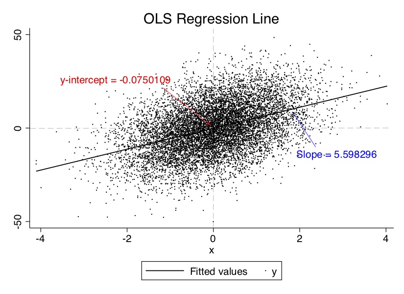
             label = "Slope = {}".format(5.685033))

Let’s look at the output from this. First, if you summarize the data, you’ll see that the fitted values are produced both using Stata’s Predict command and manually using the Generate command. I wanted the reader to have a chance to better understand this, so did it both ways. But second, let’s look at the data and paste on top of it the estimated coefficients, the y-intercept and slope on $x$ in Figure 2.1. The estimated coefficients in both are close to the hard coded values built into the data-generating process.

Figure 2.1: Graphical representation of bivariate regression from $y$ on $x$

Once we have the estimated coefficients and we have the OLS regression line, we can predict $y$ (outcome) for any (sensible) value of $x$. So plug in certain values of $x$, and we can immediately calculate what $y$ will probably be with some error. The value of OLS here lies in how large that error is: OLS minimizes the error for a linear function. In fact, it is the best such guess at $y$ for all linear estimators because it minimizes the prediction error. There’s always prediction error, in other words, with any estimator, but OLS is the least worst.

Notice that the intercept is the predicted value of $y$ if and when $x=0$. In this sample, that value is $-0.0750109$.¹² The slope allows us to predict changes in $y$ for any reasonable change in $x$ according to:

\[ \Delta \widehat{y}=\widehat{\beta}_1 \Delta x \] And if $\Delta x=1$, then $x$ increases by one unit, and so $\Delta \widehat{y}=5.598296$ in our numerical example because $\widehat{\beta}_1=5.598296$.

Now that we have calculated $\widehat{\beta}_0$ and $\widehat{\beta}_1$, we get the OLS fitted values by plugging $x_i$ into the following equation for $i=1,\dots,n$:

\[ \widehat{y_i}=\widehat{\beta}_0+\widehat{\beta}_1x_i \] The OLS residuals are also calculated by:

\[ \widehat{u_i}=y_i - \widehat{\beta}_0 - \widehat{\beta}_1 x_i \] Most residuals will be different from 0 (i.e., they do not lie on the regression line). You can see this in Figure 2.1. Some are positive, and some are negative. A positive residual indicates that the regression line (and hence, the predicted values) underestimates the true value of $y_i$. And if the residual is negative, then the regression line overestimates the true value.

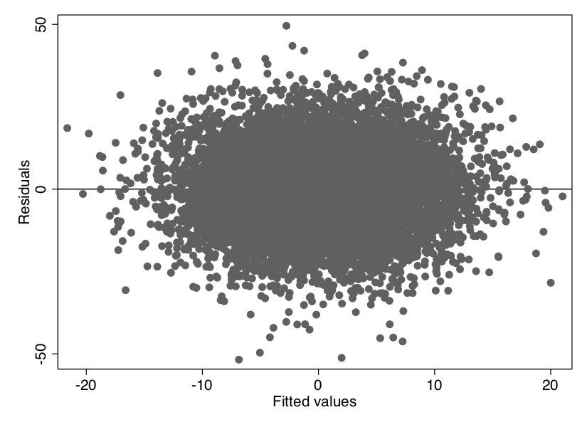
Recall that we defined the fitted value as $\widehat{y_i}$ and the residual, $\widehat{u_i}$, as $y_i - \widehat{y_i}$. Notice that the scatter-plot relationship between the residuals and the fitted values created a spherical pattern, suggesting that they are not correlated (Figure 2.2). This is mechanical—least squares produces residuals which are uncorrelated with fitted values. There’s no magic here, just least squares.

Figure 2.2: Distribution of residuals around regression line

2.14 Algebraic Properties of OLS

Remember how we obtained $\widehat{\beta}_0$ and $\widehat{\beta}_1$? When an intercept is included, we have:

\[\begin{align} \sum_{i=1}^n\Big(y_i-\widehat{\beta}_0 -\widehat{\beta}_1x_i\Big) =0 \end{align}\] The OLS residual always adds up to zero, by construction. \[ \sum_{i=1}^n \widehat{u_i}=0 \tag{2.18}\] Sometimes seeing is believing, so let’s look at this together. Type the following into Stata verbatim.

ols2.do

Code

clear 
set seed 1234
set obs 10
gen x = 9*rnormal() 
gen u  = 36*rnormal() 
gen y  = 3 + 2*x + u
reg y x
predict yhat
predict residuals, residual
su residuals
list
collapse (sum) x u y yhat residuals
list

ols2.R

Code

library(tidyverse)

set.seed(1)

tb <- tibble(
  x = 9*rnorm(10),
  u = 36*rnorm(10),
  y = 3 + 2*x + u,
  yhat = predict(lm(y ~ x)),
  uhat = residuals(lm(y ~ x))
)

summary(tb)
colSums(tb)

ols2.py

Code

import numpy as np 
import pandas as pd 
import statsmodels.api as sm 
import statsmodels.formula.api as smf 
from itertools import combinations 
import plotnine as p

# read data
import ssl
ssl._create_default_https_context = ssl._create_unverified_context
def read_data(file): 
    return pd.read_stata("https://github.com/scunning1975/mixtape/raw/master/" + file)


tb = pd.DataFrame({
    'x': 9*np.random.normal(size=10),
    'u': 36*np.random.normal(size=10)})
tb['y'] = 3*tb['x'].values + 2*tb['u'].values

reg_tb = sm.OLS.from_formula('y ~ x', data=tb).fit()

tb['yhat1'] = reg_tb.predict(tb)
tb['uhat1'] = reg_tb.resid

tb.describe()

Output from this can be summarized as in the following table (Table 2.6).

Table 2.6: Simulated data showing the sum of residuals equals zero

no.	$x$	$u$	$y$	$\widehat{y}$	$\widehat{u}$	$x\widehat{u}$	$\widehat{y}\widehat{u}$
1.	$-4.381653$	$-32.95803$	$-38.72134$	$-3.256034$	$-35.46531$	155.3967	115.4762
2.	$-13.28403$	$-8.028061$	$-31.59613$	$-26.30994$	$-5.28619$	70.22192	139.0793
3.	$-.0982034$	17.80379	20.60738	7.836532	12.77085	$-1.254141$	100.0792
4.	$-.1238423$	$-9.443188$	$-6.690872$	7.770137	$-14.46101$	1.790884	$-112.364$
5.	4.640209	13.18046	25.46088	20.10728	5.353592	24.84179	107.6462
6.	$-1.252096$	$-34.64874$	$-34.15294$	4.848374	$-39.00131$	48.83337	$-189.0929$
7.	11.58586	9.118524	35.29023	38.09396	$-2.80373$	$-32.48362$	$-106.8052$
8.	$-5.289957$	82.23296	74.65305	$-5.608207$	80.26126	$-424.5786$	$-450.1217$
9.	$-.2754041$	11.60571	14.0549	7.377647	6.677258	$-1.838944$	49.26245
10.	$-19.77159$	$-14.61257$	$-51.15575$	$-43.11034$	$-8.045414$	159.0706	346.8405
Sum	$-28.25072$	34.25085	7.749418	7.749418	1.91e-06	$-6.56e-06$	.0000305

Notice the difference between the $u$, $\widehat{y}$, and $\widehat{u}$ columns. When we sum these ten lines, neither the error term nor the fitted values of $y$ sum to zero. But the residuals do sum to zero. This is, as we said, one of the algebraic properties of OLS—coefficients were optimally chosen to ensure that the residuals sum to zero.

Because $y_i=\widehat{y_i}+\widehat{u_i}$ by definition (which we can also see in Table 6), we can take the sample average of both sides:

\[ \dfrac{1}{n} \sum_{i=1}^n y_i=\dfrac{1}{n} \sum_{i=1}^n \widehat{y_i}+\dfrac{1}{n} \sum_{i=1}^n \widehat{u_i} \] and so $\overline{y}=\overline{\widehat{y}}$ because the residuals sum to zero. Similarly, the way that we obtained our estimates yields

\[ \sum_{i=1}^n x_i \Big(y_i-\widehat{\beta}_0 - \widehat{\beta}_1 x_i\Big)=0 \] The sample covariance (and therefore the sample correlation) between the explanatory variables and the residuals is always zero (see Table 2.6).

\[ \sum_{i=1}^n x_i \widehat{u_i}=0 \] Because the $\widehat{y_i}$ are linear functions of the $x_i$, the fitted values and residuals are uncorrelated too (see Table 2.6):

\[ \sum_{i=1}^n \widehat{y_i} \widehat{u_i}=0 \tag{2.19}\] Both properties hold by construction. In other words, $\widehat{\beta}_0$ and $\widehat{\beta}_1$ were selected to make them true.¹³

A third property is that if we plug in the average for $x$, we predict the sample average for $y$. That is, the point $(\overline{x}, \overline{y})$ is on the OLS regression line, or:

\[\begin{align} \overline{y}=\widehat{\beta}_0+\widehat{\beta}_1 \overline{x} \end{align}\]

2.15 Goodness-of-fit

For each observation, we write

\[\begin{align} y_i=\widehat{y_i}+\widehat{u_i} \end{align}\] Define the total sum of squares (SST), explained sum of squares (SSE), and residual sum of squares (SSR) as

\[ SST = \sum_{i=1}^n (y_i - \overline{y})^2 \tag{2.20}\] \[ SSE = \sum_{i=1}^n (\widehat{y_i} - \overline{y})^2 \tag{2.21}\] \[ SSR = \sum_{i=1}^n \widehat{u_i}^2 \tag{2.22}\]

These are sample variances when divided by $n-1$.¹⁴ $\dfrac{SST}{n-1}$ is the sample variance of $y_i$, $\dfrac{SSE}{n-1}$ is the sample variance of $\widehat{y_i}$, and $\dfrac{SSR}{n-1}$ is the sample variance of $\widehat{u_i}$. With some simple manipulation rewrite Equation 2.20:

\[\begin{align} SST & = \sum_{i=1}^n (y_i - \overline{y})^2 \\ & = \sum_{i=1}^n \Big[ (y_i - \widehat{y_i}) + (\widehat{y_i} - \overline{y}) \Big]^2 \\ & = \sum_{i=1}^n \Big[ \widehat{u_i} + (\widehat{y_i} - \overline{y})\Big]^2 \end{align}\] Since Equation 2.19 shows that the fitted values are uncorrelated with the residuals, we can write the following equation:

\[\begin{align} SST = SSE + SSR \end{align}\] Assuming $SST>0$, we can define the fraction of the total variation in $y_i$ that is explained by $x_i$ (or the OLS regression line) as

\[\begin{align} R^2=\dfrac{SSE}{SST}=1-\dfrac{SSR}{SST} \end{align}\] which is called the R-squared of the regression. It can be shown to be equal to the square of the correlation between $y_i$ and $\widehat{y_i}$. Therefore $0\leq R^2 \leq 1$. An R-squared of zero means no linear relationship between $y_i$ and $x_i$, and an $R$-squared of one means a perfect linear relationship (e.g., $y_i=x_i+2$). As $R^2$ increases, the $y_i$ are closer and closer to falling on the OLS regression line.

I would encourage you not to fixate on $R$-squared in research projects where the aim is to estimate some causal effect, though. It’s a useful summary measure, but it does not tell us about causality. Remember, you aren’t trying to explain variation in $y$ if you are trying to estimate some causal effect. The $R^2$ tells us how much of the variation in $y_i$ is explained by the explanatory variables. But if we are interested in the causal effect of a single variable, $R^2$ is irrelevant. For causal inference, we need Equation 2.17.

2.16 Expected value of OLS

Up until now, we motivated simple regression using a population model. But our analysis has been purely algebraic, based on a sample of data. So residuals always average to zero when we apply OLS to a sample, regardless of any underlying model. But our job gets tougher. Now we have to study the statistical properties of the OLS estimator, referring to a population model and assuming random sampling.¹⁵

The field of mathematical statistics is concerned with questions. How do estimators behave across different samples of data? On average, for instance, will we get the right answer if we repeatedly sample? We need to find the expected value of the OLS estimators—in effect, the average outcome across all possible random samples—and determine whether we are right, on average. This leads naturally to a characteristic called unbiasedness, which is desirable of all estimators. \[ E(\widehat{\beta})=\beta \tag{2.23}\] Remember, our objective is to estimate $\beta_1$, which is the slope ${population}$ parameter that describes the relationship between $y$ and $x$. Our estimate, $\widehat{\beta_1}$, is an estimator of that parameter obtained for a specific sample. Different samples will generate different estimates ($\widehat{\beta_1}$) for the “true” (and unobserved) $\beta_1$. Unbiasedness means that if we could take as many random samples on $Y$ as we want from the population and compute an estimate each time, the average of the estimates would be equal to $\beta_1$.

There are several assumptions required for OLS to be unbiased. The first assumption is called linear in the parameters. Assume a population model

\[ y=\beta_0+\beta_1 x+u \] where $\beta_0$ and $\beta_1$ are the unknown population parameters. We view $x$ and $u$ as outcomes of random variables generated by some data-generating process. Thus, since $y$ is a function of $x$ and $u$, both of which are random, then $y$ is also random. Stating this assumption formally shows that our goal is to estimate $\beta_0$ and $\beta_1$.

Our second assumption is random sampling. We have a random sample of size $n$, $\{ (x_i, y_i){:} i=1, \dots, n\}$, following the population model. We know how to use this data to estimate $\beta_0$ and $\beta_1$ by OLS. Because each $i$ is a draw from the population, we can write, for each $i$:

\[ y_i=\beta_0+\beta_1x_i+u_i \] Notice that $u_i$ here is the unobserved error for observation $i$. It is not the residual that we compute from the data.

The third assumption is called sample variation in the explanatory variable. That is, the sample outcomes on $x_i$ are not all the same value. This is the same as saying that the sample variance of $x$ is not zero. In practice, this is no assumption at all. If the $x_i$ all have the same value (i.e., are constant), we cannot learn how $x$ affects $y$ in the population. Recall that OLS is the covariance of $y$ and $x$ divided by the variance in $x$, and so if $x$ is constant, then we are dividing by zero, and the OLS estimator is undefined.

With the fourth assumption our assumptions start to have real teeth. It is called the zero conditional mean assumption and is probably the most critical assumption in causal inference. In the population, the error term has zero mean given any value of the explanatory variable:

\[ E(u\mid x) = E(u) = 0 \tag{2.24}\] This is the key assumption for showing that OLS is unbiased, with the zero value being of no importance once we assume that $E(u\mid x)$ does not change with $x$. Note that we can compute OLS estimates whether or not this assumption holds, even if there is an underlying population model.

So, how do we show that $\widehat{\beta_1}$ is an unbiased estimate of $\beta_1$ (Equation 2.24)? We need to show that under the four assumptions we just outlined, the expected value of $\widehat{\beta_1}$, when averaged across random samples, will center on the true value of $\beta_1$. This is a subtle yet critical concept. Unbiasedness in this context means that if we repeatedly sample data from a population and run a regression on each new sample, the average over all those estimated coefficients will equal the true value of $\beta_1$. We will discuss the answer as a series of steps.

Step 1: Write down a formula for $\widehat{\beta_1}$. It is convenient to use the $\dfrac{C(x,y)}{V(x)}$ form:

\[\begin{align} \widehat{\beta_1}=\dfrac{\sum_{i=1}^n (x_i - \overline{x})y_i}{\sum_{i=1}^n (x_i - \overline{x})^2} \end{align}\] Let’s get rid of some of this notational clutter by defining $\sum_{i=1}^n (x_i - \overline{x})^2=SST_x$ (i.e., total variation in the $x_i$) and rewrite this as:

\[\begin{align} \widehat{\beta_1}=\dfrac{ \sum_{i=1}^n (x_i - \overline{x})y_i}{SST_x} \end{align}\]

Step 2: Replace each $y_i$ with $y_i= \beta_0+\beta_1 x_i+u_i$, which uses the first linear assumption and the fact that we have sampled data (our second assumption). The numerator becomes:

\[\begin{align} \sum_{i=1}^n (x_i - \overline{x})y_i & =\sum_{i=1}^n (x_i - \overline{x})(\beta_0+\beta_1 x_i+u_i) \\ & = \beta_0 \sum_{i=1}^n (x_i - \overline{x})+\beta_1 \sum_{i=1}^n (x_i - \overline{x})x_i+\sum_{i=1}^n (x_i+\overline{x}) u_i \\ & =0+\beta_1 \sum_{i=1}^n (x_i - \overline{x})^2+ \sum_{i=1}^n (x_i - \overline{x})u_i \\ & = \beta_1 SST_x+\sum_{i=1}^n (x_i - \overline{x}) u_i \end{align}\] Note, we used $\sum_{i=1}^n (x_i-\overline{x})=0$ and $\sum_{i=1}^n (x_i - \overline{x})x_i=\sum_{i=1}^n (x_i - \overline{x})^2$ to do this.¹⁶

We have shown that:

\[\begin{align} \widehat{\beta_1} & = \dfrac{ \beta_1 SST_x+ \sum_{i=1}^n (x_i - \overline{x})u_i }{SST_x} \nonumber \\ & = \beta_1+\dfrac{ \sum_{i=1}^n (x_i - \overline{x})u_i }{SST_x} \end{align}\] Note that the last piece is the slope coefficient from the OLS regression of $u_i$ on $x_i$, $i$: $1, \dots, n$.¹⁷ We cannot do this regression because the $u_i$ are not observed. Now define $w_i=\dfrac{(x_i - \overline{x})}{SST_x}$ so that we have the following:

\[\begin{align} \widehat{\beta_1}=\beta_1+\sum_{i=1}^n w_i u_i \end{align}\] This has showed us the following: First, $\widehat{\beta_1}$ is a linear function of the unobserved errors, $u_i$. The $w_i$ are all functions of $\{ x_1, \dots, x_n \}$. Second, the random difference between $\beta_1$ and the estimate of it, $\widehat{\beta_1}$, is due to this linear function of the unobservables.

Step 3: Find $E(\widehat{\beta_1})$. Under the random sampling assumption and the zero conditional mean assumption, $E(u_i \mid x_1, \dots, x_n)=0$, that means conditional on each of the $x$ variables:

\[\begin{align} E\big(w_iu_i\mid x_1, \dots, x_n\big) = w_i E\big(u_i \mid x_1, \dots, x_n\big)=0 \end{align}\] because $w_i$ is a function of $\{x_1, \dots, x_n\}$. This would be true if in the population $u$ and $x$ are correlated.

Now we can complete the proof: conditional on $\{x_1, \dots, x_n\}$,

\[\begin{align} E(\widehat{\beta_1}) & = E \bigg(\beta_1+\sum_{i=1}^n w_i u_i \bigg) \\ & =\beta_1+\sum_{i=1}^n E(w_i u_i) \\ & = \beta_1+\sum_{i=1}^n w_i E(u_i) \\ & =\beta_1 +0 \\ & =\beta_1 \end{align}\] Remember, $\beta_1$ is the fixed constant in the population. The estimator, $\widehat{\beta_1}$, varies across samples and is the random outcome: before we collect our data, we do not know what $\widehat{\beta_1}$ will be. Under the four aforementioned assumptions, $E(\widehat{\beta_0})=\beta_0$ and $E(\widehat{\beta_1})=\beta_1$.

I find it helpful to be concrete when we work through exercises like this. So let’s visualize this. Let’s create a Monte Carlo simulation. We have the following population model:

\[ y=3+2x+u \tag{2.25}\] where $x\sim Normal(0,9)$, $u\sim Normal(0,36)$. Also, $x$ and $u$ are independent. The following Monte Carlo simulation will estimate OLS on a sample of data 1,000 times. The true $\beta$ parameter equals 2. But what will the average $\widehat{\beta}$ equal when we use repeated sampling?

ols3.do

Code

clear all 
program define ols, rclass 
version 14.2 
syntax [, obs(integer 1) mu(real 0) sigma(real 1) ] 

    clear 
    drop _all 
    set obs 10000 
    gen x = 9*rnormal()  
    gen u  = 36*rnormal()  
    gen y  = 3 + 2*x + u 
    reg y x 
    end 

simulate beta=_b[x], reps(1000): ols 
su 
hist beta

ols3.R

Code

library(tidyverse)

lm <- lapply(
  1:1000,
  function(x) tibble(
    x = 9*rnorm(10000),
    u = 36*rnorm(10000),
    y = 3 + 2*x + u
  ) %>% 
    lm(y ~ x, .)
)

as_tibble(t(sapply(lm, coef))) %>%
  summary(x)

as_tibble(t(sapply(lm, coef))) %>% 
  ggplot()+
  geom_histogram(aes(x), binwidth = 0.01)

ols3.py

Code

import numpy as np 
import pandas as pd 
import statsmodels.api as sm 
import statsmodels.formula.api as smf 
from itertools import combinations 
import plotnine as p

# read data
import ssl
ssl._create_default_https_context = ssl._create_unverified_context
def read_data(file): 
    return pd.read_stata("https://github.com/scunning1975/mixtape/raw/master/" + file)

coefs = np.zeros(1000)
for i in range(1000):
    tb = pd.DataFrame({
    'x': 9*np.random.normal(size=10000),
    'u': 36*np.random.normal(size=10000)})
    tb['y'] = 3 + 2*tb['x'].values + tb['u'].values

    reg_tb = sm.OLS.from_formula('y ~ x', data=tb).fit()

    coefs[i] = reg_tb.params['x']

p.ggplot() +\
  p.geom_histogram(p.aes(x=coefs), binwidth = 0.01)

Table 2.7: Monte Carlo simulation of OLS.

Variable	Obs	Mean	St. Dev.
beta	1,000	1.998317	0.0398413

Table 2.7 gives us the mean value of $\widehat{\beta-1}$ over the 1,000 repetitions (repeated sampling). Your results will differ from mine here only in the randomness involved in the simulation. But your results should be similar to what is shown here. While each sample had a different estimated slope, the average for $\widehat{\beta-1}$ over all the samples was 1.998317, which is close to the true value of 2 (see Equation 2.25). The standard deviation in this estimator was 0.0398413, which is close to the standard error recorded in the regression itself.¹⁸ Thus, we see that the estimate is the mean value of the coefficient from repeated sampling, and the standard error is the standard deviation from that repeated estimation. We can see the distribution of these coefficient estimates in Figure 2.3.

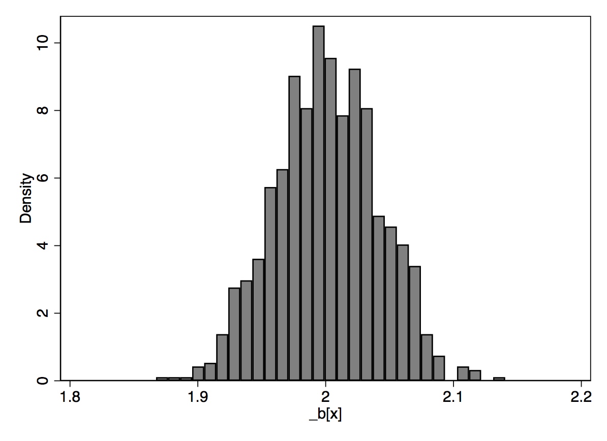
Figure 2.3: Distribution of coefficients from Monte Carlo simulation.

The problem is, we don’t know which kind of sample we have. Do we have one of the “almost exactly 2” samples, or do we have one of the “pretty different from 2” samples? We can never know whether we are close to the population value. We hope that our sample is “typical” and produces a slope estimate close to $\widehat{\beta_1}$, but we can’t know. Unbiasedness is a property of the procedure of the rule. It is not a property of the estimate itself. For example, say we estimated an that 8.2% return on schooling. It is tempting to say that 8.2% is an unbiased estimate of the return to schooling, but that’s technically incorrect. The rule used to get $\widehat{\beta_1}=0.082$ is unbiased (if we believe that $u$ is unrelated to schooling), not the actual estimate itself.

2.17 Law of iterated expectations

The conditional expectation function (CEF) is the mean of some outcome $y$ with some covariate $x$ held fixed. Let’s focus more intently on this function.¹⁹ Let’s get the notation and some of the syntax out of the way. As noted earlier, we write the CEF as $E(y_i\mid x_i)$. Note that the CEF is explicitly a function of $x_i$. And because $x_i$ is random, the CEF is random—although sometimes we work with particular values for $x_i$, like $E(y_i\mid x_i=8\text{ years schooling})$ or $E(y_i\mid x_i=\text{Female})$. When there are treatment variables, then the CEF takes on two values: $E(y_i\mid d_i=0)$ and $E(y_i\mid d_i= 1)$. But these are special cases only.

An important complement to the CEF is the law of iterated expectations (LIE). This law says that an unconditional expectation can be written as the unconditional average of the CEF. In other words, $E(y_i)=E \{E(y_i\mid x_i)\}$. This is a fairly simple idea: if you want to know the unconditional expectation of some random variable $y$, you can simply calculate the weighted sum of all conditional expectations with respect to some covariate $x$. Let’s look at an example. Let’s say that average grade-point for females is 3.5, average GPA for males is a 3.2, half the population is female, and half is male. Then:

\[\begin{align} E[GPA] & = E \big\{E(GPA_i\mid \text{Gender}_i) \big\} \\ & =(0.5 \times 3.5)+(3.2 \times 0.5) \\ & = 3.35 \end{align}\] You probably use LIE all the time and didn’t even know it. The proof is not complicated. Let $x_i$ and $y_i$ each be continuously distributed. The joint density is defined as $f_{xy}(u,t)$. The conditional distribution of $y$ given $x=u$ is defined as $f_y(t\mid x_i=u)$. The marginal densities are $g_y(t)$ and $g_x(u)$.

\[\begin{align} E \{E(y\mid x)\} & = \int E(y\mid x=u) g_x(u) du \\ & = \int \bigg[ \int tf_{y\mid x} (t\mid x=u) dt \bigg] g_x(u) du \\ & = \int \int t f_{y\mid x} (t\mid x=u) g_x(u) du dt \\ & = \int t \bigg[ \int f_{y\mid x} (t\mid x=u) g_x(u) du \bigg] dt \text{} \\ & = \int t [ f_{x,y}du] dt \\ & = \int t g_y(t) dt \\ & =E(y) \end{align}\] Check out how easy this proof is. The first line uses the definition of expectation. The second line uses the definition of conditional expectation. The third line switches the integration order. The fourth line uses the definition of joint density. The fifth line replaces the prior line with the subsequent expression. The sixth line integrates joint density over the support of x which is equal to the marginal density of $y$. So restating the law of iterated expectations: $E(y_i)= E\{E(y\mid x_i)\}$.

2.18 CEF decomposition property

The first property of the CEF we will discuss is the CEF decomposition property. The power of LIE comes from the way it breaks a random variable into two pieces—the CEF and a residual with special properties. The CEF decomposition property states that \[ y_i=E(y_i\mid x_i)+\varepsilon_i\ \]

where (i) $\varepsilon_i$ is mean independent of $x_i$, That is,

\[ E(\varepsilon_i\mid x_i)=0 \]

and (ii) $\varepsilon_i$ is not correlated with any function of $x_i$.

The theorem says that any random variable $y_i$ can be decomposed into a piece that is explained by $x_i$ (the CEF) and a piece that is left over and orthogonal to any function of $x_i$. I’ll prove the (i) part first. Recall that $\varepsilon_i=y_i - E(y_i\mid x_i)$ as we will make a substitution in the second line below.

\[\begin{align} E(\varepsilon_i\mid x_i) & =E\Big(y_i- E(y_i\mid x_i)\mid x_i\Big) \\ & =E(y_i\mid x_i) - E(y_i\mid x_i) \\ & = 0 \end{align}\]

The second part of the theorem states that $\varepsilon_i$ is uncorrelated with any function of $x_i$. Let $h(x_i)$ be any function of $x_i$. Then $E( h(x_i) \varepsilon_i)=E \{ h(x_i) E(\varepsilon_i\mid x_i)\}$ The second term in the interior product is equal to zero by mean independence.²⁰

2.19 CEF prediction property

The second property is the CEF prediction property. This states that $E(y_i\mid x_i)=\arg\min_{m(x_i)}E[(y-m(x_i))^2]$, where $m(x_i)$ is any function of $x_i$. In words, this states that the CEF is the minimum mean squared error of $y_i$ given $x_i$. By adding $E(y_i\mid x_i) - E(y_i\mid x_i)=0$ to the right side we get \[ \Big[y_i-m(x_i)\Big]^2=\Big[\big(y_i-E[y_i\mid x_i]\big) +\big(E(y_i\mid x_i)- m(x_i)\big)\Big]^2 \] I personally find this easier to follow with simpler notation. So replace this expression with the following terms: \[ (a-b+b-c)^2 = (a-b)^2 + 2 (b-c)(a-b) + (b-c)^2 \] Distribute the terms, rearrange them, and replace the terms with their original values until you get the following:

\[\begin{align} \arg\min \Big(y_i- E(y_i\mid x_i)\Big)^2 & + 2\Big(E(y_i\mid x_i)- m(x_i)\Big)\times \Big(y_i - E(y_i\mid x_i)\Big)\\ & +\Big(E(y_i\mid x_i)+m(x_i)\Big)^2 \end{align}\]

Now minimize the function with respect to $m(x_i)$. When minimizing this function with respect to $m(x_i)$, note that the first term $(y_i-E(y_i\mid x_i))^2$ doesn’t matter because it does not depend on $m(x_i)$. The second and third terms, though, do depend on $m(x_i)$. So rewrite $2(E (y_i\mid x_i)-m(x_i))$ as $h(x_i)$. Also set $\varepsilon_i$ equal to $[y_i-E(y_i\mid x_i)]$ and substitute \[ \arg\min\varepsilon_i^2+h(x_i)\varepsilon_i+ \Big[ E(y_i\mid x_i)+m(x_i)\Big]^2 \] Now minimizing this function and setting it equal to zero we get \[ h'(x_i)\varepsilon_i \] which equals zero by the decomposition property.

2.20 ANOVA theory

The final property of the CEF that we will discuss is the analysis of variance theorem, or ANOVA. According to this theorem, the unconditional variance in some random variable is equal to the variance in the conditional expectation plus the expectation of the conditional variance, or \[ V(y_i)=V\Big[E(y_i\mid x_i)\Big]+ E\Big[V(y_i\mid x_i)\Big] \] where $V$ is the variance and $V(y_i\mid x_i)$ is the conditional variance.

2.21 Linear CEF theorem

As you probably know by now, the use of least squares in applied work is extremely common. That’s because regression has several justifications. We discussed one—unbiasedness under certain assumptions about the error term. But I’d like to present some slightly different arguments. Angrist and Pischke (2009) argue that linear regression may be useful even if the underlying CEF itself is not linear, because regression is a good approximation of the CEF. So keep an open mind as I break this down a little bit more.

Angrist and Pischke (2009) give several arguments for using regression, and the linear CEF theorem is probably the easiest. Let’s assume that we are sure that the CEF itself is linear. So what? Well, if the CEF is linear, then the linear CEF theorem states that the population regression is equal to that linear CEF. And if the CEF is linear, and if the population regression equals it, then of course you should use the population regression to estimate CEF. If you need a proof for what could just as easily be considered common sense, I provide one. If $E(y_i\mid x_i)$ is linear, then $E(y_i\mid x_i)= x'\widehat{\beta}$ for some vector $\widehat{\beta}$. By the decomposition property, you get: \[ E\Big(x(y-E(y\mid x)\Big)=E\Big(x(y-x'\widehat{\beta})\Big)=0 \] And then when you solve this, you get $\widehat{\beta}=\beta$. Hence $E(y\mid x)=x'\beta$.

2.22 Best linear predictor theorem

There are a few other linear theorems that are worth bringing up in this context. For instance, recall that the CEF is the minimum mean squared error predictor of $y$ given $x$ in the class of all functions, according to the CEF prediction property. Given this, the population regression function is the best that we can do in the class of all linear functions.²¹

2.23 Regression CEF theorem

I would now like to cover one more attribute of regression. The function $X\beta$ provides the minimum mean squared error linear approximation to the CEF. That is, \[ \beta=\arg\min_b E\Big\{\big[E(y_i\mid x_i) - x_i'b\big]^2 \Big\} \] So? Let’s try and back up for a second, though, and get the big picture, as all these linear theorems can leave the reader asking, “So what?” I’m telling you all of this because I want to present to you an argument that regression is appealing; even though it’s linear, it can still be justified when the CEF itself isn’t. And since we don’t know with certainty that the CEF is linear, this is actually a nice argument to at least consider. Regression is ultimately nothing more than a crank turning data into estimates, and what I’m saying here is that crank produces something desirable even under bad situations. Let’s look a little bit more at this crank, though, by reviewing another theorem which has become popularly known as the regression anatomy theorem.

2.24 Regression anatomy theorem

In addition to our discussion of the CEF and regression theorems, we now dissect the regression itself. Here we discuss the regression anatomy theorem. The regression anatomy theorem is based on earlier work by Frisch and Waugh (1933) and Lovell (1963).²² I find the theorem more intuitive when I think through a specific example and offer up some data visualization. I have found Filoso (2013) very helpful in explaining this with proofs and algebraic derivations, so I will use this notation and set of steps here as well. In my opinion, the theorem helps us interpret the individual coefficients of a multiple linear regression model. Say that we are interested in the causal effect of family size on labor supply. We want to regress labor supply on family size:

\[\begin{align} Y_i=\beta_0+\beta_1 X_i+u_i \end{align}\] where $Y$ is labor supply, and $X$ is family size.

If family size is truly random, then the number of kids in a family is uncorrelated with the unobserved error term.²³ This implies that when we regress labor supply on family size, our estimate, $\widehat{\beta}_1$, can be interpreted as the causal effect of family size on labor supply. We could just plot the regression coefficient in a scatter plot showing all $i$ pairs of data; the slope coefficient would be the best linear fit of the data for this data cloud. Furthermore, under randomized number of children, the slope would also tell us the average causal effect of family size on labor supply.

But most likely, family size isn’t random, because so many people choose the number of children to have in their family—instead of, say, flipping a coin. So how do we interpret $\widehat{\beta}_1$ if the family size is not random? Often, people choose their family size according to something akin to an optimal stopping rule. People pick both how many kids to have, when to have them, and when to stop having them. In some instances, they may even attempt to pick the gender. All of these choices are based on a variety of unobserved and observed economic factors that may themselves be associated with one’s decision to enter the labor market. In other words, using the language we’ve been using up until now, it’s unlikely that $E(u\mid X)=E(u)=0$.

But let’s say that we have reason to think that the number of kids in a family is conditionally random. To make this tractable for the sake of pedagogy, let’s say that a particular person’s family size is as good as randomly chosen once we condition on race and age.²⁴ While unrealistic, I include it to illustrate an important point regarding multivariate regressions. If this assumption were to be true, then we could write the following equation:

\[\begin{align} Y_i=\beta_0+\beta_1 X_i+\gamma_1 R_i+\gamma_2A_i+u_i \end{align}\] where $Y$ is labor supply, $X$ is number of kids, $R$ is race, $A$ is age, and $u$ is the population error term.

If we want to estimate the average causal effect of family size on labor supply, then we need two things. First, we need a sample of data containing all four of those variables. Without all four of the variables, we cannot estimate this regression model. Second, we need for the number of kids, $X$, to be randomly assigned for a given set of race and age.

Now, how do we interpret $\widehat{\beta}_1$? And how might we visualize this coefficient given that there are six dimensions to the data? The regression anatomy theorem both tells us what this coefficient estimate actually means and also lets us visualize the data in only two dimensions.

To explain the intuition of the regression anatomy theorem, let’s write down a population model with multiple variables. Assume that your main multiple regression model of interest has K covariates. We can then write it as: \[ y_i=\beta_0+\beta_1 x_{1i}+\dots+\beta_k x_{ki}+ \dots+\beta_K x_{Ki}+e_i \] Now assume an auxiliary regression in which the variable $x_{1i}$ is regressed on all the remaining independent variables: \[ x_{1i}=\gamma_0+\gamma_{k-1}x_{k-1i}+ \gamma_{k+1}x_{k+1i}+\dots+\gamma_Kx_{Ki}+f_i \] and $\tilde{x}_{1i}=x_{1i} - \widehat{x}_{1i}$ is the residual from that auxiliary regression. Then the parameter $\beta_1$ can be rewritten as: \[ \beta_1=\dfrac{C(y_i,\tilde{x}_i)}{V(\tilde{x}_i)} \] Notice that again we see that the coefficient estimate is a scaled covariance, only here, the covariance is with respect to the outcome and residual from the auxiliary regression, and the scale is the variance of that same residual.

To prove the theorem, note that $E[\tilde{x}_{ki}]=E[x_{ki}] - E[\widehat{x}_{ki}]=E[f_i]$, and plug $y_i$ and residual $\tilde{x}_{ki}$ from $x_{ki}$ auxiliary regression into the covariance $\cov(y_i,x_{ki})$:

\[\begin{align} \beta_k & = \dfrac{\cov( \beta_0+\beta_1 x_{1i}+\dots+ \beta_kx_{ki}+\dots+\beta_Kx_{Ki}+e_i, \tilde{x}_{ki})}{\var(\tilde{x}_{ki})} \\ & = \dfrac{\cov(\beta_0+\beta_1 x_{1i}+\dots+\beta_k x_{ki}+\dots+\beta_K x_{Ki}+e_i, f_i)}{\var(f_i)} \end{align}\]

Since by construction $E[f_i]=0$, it follows that the term $\beta_0 E[f_i]=0$. Since $f_i$ is a linear combination of all the independent variables with the exception of $x_{ki}$, it must be that

\[\begin{align} \beta_1E[f_ix_{1i}]=\dots=\beta_{k-1}E[f_ix_{k-1i}]= \beta_{k+1} E[f_ix_{k+1i}]=\dots=\beta_K E[f_ix_{Ki}]=0 \end{align}\]

Consider now the term $E[e_if_i]$. This can be written as

\[\begin{align} E[e_if_i] & = E[e_i \tilde{x}_{ki}] \\ & = E\Big[e_i(x_{ki}-\widehat{x}_{ki})\Big] \\ & = E[e_ix_{ki}]-E[e_i\tilde{x}_{ki}] \end{align}\]

Since $e_i$ is uncorrelated with any independent variable, it is also uncorrelated with $x_{ki}$. Accordingly, we have $E[e_ix_{ki}]=0$. With regard to the second term of the subtraction, substituting the predicted value from the $x_{ki}$ auxiliary regression, we get \[ E[e_i\tilde{x}_{ki}]=E\Big[e_i(\widehat{\gamma}_0+ \widehat{\gamma}_1x_{1i}+\dots+ \widehat{\gamma}_{k-1i}+ \widehat{\gamma}_{k+1}x_{k+1i}+\dots+ \widehat{x}_Kx_{Ki})\Big] \]

Once again, since $e_i$ is uncorrelated with any independent variable, the expected value of the terms is equal to zero. It follows that $E[e_if_i]=0$.

The only remaining term, then, is $[\beta_kx_{ki}f_i]$, which equals $E[\beta_kx_{ki}\tilde{x}_{ki}]$, since $f_i=\tilde{x}_{ki}$. The term $x_{ki}$ can be substituted by rewriting the auxiliary regression model, $x_{ki}$, such that

\[\begin{align} x_{ki}=E[x_{ki}\mid X_{-k}]+\tilde{x}_{ki} \end{align}\]

This gives

\[\begin{align} E[\beta_{k}x_{ki}\tilde{x}_{ki}] & = \beta_k E\Big[\tilde{x}_{ki} ( E[x_{ki}\mid X_{-k}]+ \tilde{x}_{ki})\Big] \\ & = \beta_k \Big\{ E[\tilde{x}_{ki}^2]+ E[(E[x_{ki}\mid x_{-k}]\tilde{x}_{ki})]\Big\} \\ & = \beta_{k}\var(\tilde{x}_{ki}) \end{align}\]

which follows directly from the orthogonality between $E[x_{ki}\mid X_{-k}]$ and $\tilde{x}_{ki}$. From previous derivations we finally get \[ \cov(y_i,\tilde{x}_{ki})=\beta_k\var(\tilde{x}_{ki}) \] which completes the proof.

I find it helpful to visualize things. Let’s look at an example in Stata using its popular automobile data set. I’ll show you:

reganat.do

Code

* -reganat- is a user-created package by @Filoso2013. 
ssc install reganat, replace
sysuse auto.dta, replace
regress price length
regress price length weight headroom mpg
reganat price length weight headroom mpg, dis(length) biline

reganat.R

Code

library(tidyverse)
library(haven)

read_data <- function(df) {
  full_path <- paste0("https://github.com/scunning1975/mixtape/raw/master/",
                      df)
  haven::read_dta(full_path)
}

auto <-
  read_data("auto.dta") %>%
  mutate(length = length - mean(length))

lm1 <- lm(price ~ length, auto)
lm2 <- lm(price ~ length + weight + headroom + mpg, auto)
lm_aux <- lm(length ~ weight + headroom + mpg, auto)
auto <-
  auto %>%
  mutate(length_resid = residuals(lm_aux))

lm2_alt <- lm(price ~ length_resid, auto)

coef_lm1 <- lm1$coefficients
coef_lm2_alt <- lm2_alt$coefficients
resid_lm2 <- lm2$residuals

y_single <- tibble(price = coef_lm2_alt[1] + coef_lm1[2]*auto$length_resid,
                   length_resid = auto$length_resid)

y_multi <- tibble(price = coef_lm2_alt[1] + coef_lm2_alt[2]*auto$length_resid,
                  length_resid = auto$length_resid)

auto %>%
  ggplot(aes(x=length_resid, y = price)) +
  geom_point() +
  geom_smooth(data = y_multi, color = "blue") +
  geom_smooth(data = y_single, color = "red")

reganat.py

Code

import numpy as np 
import pandas as pd 
import statsmodels.api as sm 
import statsmodels.formula.api as smf 
from itertools import combinations 
import plotnine as p

# read data
import ssl
ssl._create_default_https_context = ssl._create_unverified_context
def read_data(file): 
    return pd.read_stata("https://github.com/scunning1975/mixtape/raw/master/" + file)


auto = pd.read_stata('https://github.com/scunning1975/mixtape/raw/master/auto.dta')
auto['length'] = auto['length'] - auto['length'].mean()

lm1 = sm.OLS.from_formula('price ~ length', data=auto).fit()
lm2 = sm.OLS.from_formula('price ~ length + weight + headroom + mpg', data=auto).fit()


coef_lm1 = lm1.params
coef_lm2 = lm2.params
resid_lm2 = lm2.resid

auto['y_single'] = coef_lm1[0] + coef_lm1[1]*auto['length']
auto['y_multi'] = coef_lm1[0] + coef_lm2[1]*auto['length']

p.ggplot(auto) +\
  p.geom_point(p.aes(x = 'length', y = 'price')) +\
  p.geom_smooth(p.aes(x = 'length', y = 'y_multi'), color = "blue") +\
  p.geom_smooth(p.aes(x = 'length', y = 'y_single'), color="red")

Let’s walk through both the regression output that I’ve reproduced in Table 2.8 as well as a nice visualization of the slope parameters in what I’ll call the short bivariate regression and the longer multivariate regression. The short regression of price on car length yields a coefficient of 57.20 on length. For every additional inch, a car is $57 more expensive, which is shown by the upward-sloping, dashed line in Figure 2.4. The slope of that line is 57.20.

Table 2.8: Regression estimates of automobile price on length and other characteristics.

Covariates
Length	57.20	$-94.50$
	(14.08)	(40.40)
Weight		4.34
		(1.16)
Headroom		$-490.97$
		(388.49)
MPG		$-87.96$
		(83.59)

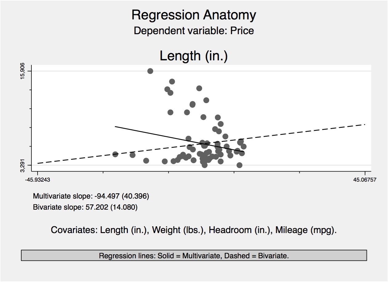
It will eventually become second nature for you to talk about including more variables on the right side of a regression as “controlling for” those variables. But in this regression anatomy exercise, I hope to give a different interpretation of what you’re doing when you in fact “control for” variables in a regression. First, notice how the coefficient on length changed signs and increased in magnitude once we controlled for the other variables. Now, the effect on length is $-94.5$. It appears that the length was confounded by several other variables, and once we conditioned on them, longer cars actually were cheaper. You can see a visual representation of this in Figure 2.4, where the multivariate slope is negative.

So what exactly going on in this visualization? Well, for one, it has condensed the number of dimensions (variables) from four to only two. It did this through the regression anatomy process that we described earlier. Basically, we ran the auxiliary regression, used the residuals from it, and then calculated the slope coefficient as $\dfrac{\cov(y_i,\tilde{x}_i)}{\var{(\tilde{x}_i)}}$. This allowed us to show scatter plots of the auxiliary residuals paired with their outcome observations and to slice the slope through them (Figure 2.4). Notice that this is a useful way to preview the multidimensional correlation between two variables from a multivariate regression. Notice that the solid black line is negative and the slope from the bivariate regression is positive. The regression anatomy theorem shows that these two estimators—one being a multivariate OLS and the other being a bivariate regression price and a residual—are identical.

2.25 Variance of the OLS estimators

That more or less summarizes what we want to discuss regarding the linear regression. Under a zero conditional mean assumption, we could epistemologically infer that the rule used to produce the coefficient from a regression in our sample was unbiased. That’s nice because it tells us that we have good reason to believe that result. But now we need to build out this epistemological justification so as to capture the inherent uncertainty in the sampling process itself. This added layer of uncertainty is often called inference. Let’s turn to it now.

Remember the simulation we ran earlier in which we resampled a population and estimated regression coefficients a thousand times? We produced a histogram of those 1,000 estimates in Figure 2.3. The mean of the coefficients was around 1.998, which was very close to the true effect of 2 (hard-coded into the data-generating process). But the standard deviation was around 0.04. This means that, basically, in repeated sampling of some population, we got different estimates. But the average of those estimates was close to the true effect, and their spread had a standard deviation of 0.04. This concept of spread in repeated sampling is probably the most useful thing to keep in mind as we move through this section.

Under the four assumptions we discussed earlier, the OLS estimators are unbiased. But these assumptions are not sufficient to tell us anything about the variance in the estimator itself. The assumptions help inform our beliefs that the estimated coefficients, on average, equal the parameter values themselves. But to speak intelligently about the variance of the estimator, we need a measure of dispersion in the sampling distribution of the estimators. As we’ve been saying, this leads us to the variance and ultimately to the standard deviation. We could characterize the variance of the OLS estimators under the four assumptions. But for now, it’s easiest to introduce an assumption that simplifies the calculations. We’ll keep the assumption ordering we’ve been using and call this the fifth assumption.

The fifth assumption is the homoskedasticity or constant variance assumption. This assumption stipulates that our population error term, $u$, has the same variance given any value of the explanatory variable, $x$. Formally, this is: \[ V(u\mid x)=\sigma^2 \] When I was first learning this material, I always had an unusually hard time wrapping my head around $\sigma^2$. Part of it was because of my humanities background; I didn’t really have an appreciation for random variables that were dispersed. I wasn’t used to taking a lot of numbers and trying to measure distances between them, so things were slow to click. So if you’re like me, try this. Think of $\sigma^2$ as just a positive number like 2 or 8. That number is measuring the spreading out of underlying errors themselves. In other words, the variance of the errors conditional on the explanatory variable is simply some finite, positive number. And that number is measuring the variance of the stuff other than $x$ that influence the value of $y$ itself. And because we assume the zero conditional mean assumption, whenever we assume homoskedasticity, we can also write: \[ E(u^2\mid x)=\sigma^2=E(u^2) \] Now, under the first, fourth, and fifth assumptions, we can write: \[\begin{align} E(y\mid x) & = \beta_0+\beta_1 x \\ V(y\mid x) & = \sigma^2 \end{align}\] So the average, or expected, value of $y$ is allowed to change with $x$, but if the errors are homoskedastic, then the variance does not change with $x$. The constant variance assumption may not be realistic; it must be determined on a case-by-case basis.

Theorem: Sampling variance of OLS. Under assumptions 1 and 2, we get:

\[\begin{align} V(\widehat{\beta_1}\mid x)&=\dfrac{\sigma^2}{\sum_{i=1}^n (x_i-\overline{x})^2}\\ &= \dfrac{ \sigma^2}{SST_x} \end{align}\]

\[ V(\widehat{\beta_0}\mid x)= \dfrac{\sigma^2\left(\dfrac{1}{n} \sum_{i=1}^n x_i^2\right)}{SST_x} \] To show this, write, as before, \[ \widehat{\beta_1}=\beta_1+ \sum_{i=1}^n w_i u_i \] where $w_i=\dfrac{(x_i-\overline{x})}{SST_x}$. We are treating this as nonrandom in the derivation. Because $\beta_1$ is a constant, it does not affect $V(\widehat{\beta_1})$. Now, we need to use the fact that, for uncorrelated random variables, the variance of the sum is the sum of the variances. The $\{ u_i: i=1, \dots, n \}$ are actually independent across $i$ and uncorrelated. Remember: if we know $x$, we know $w$. So:

\[\begin{align} V(\widehat{\beta_1}\mid x) & =\Var(\beta_1+ \sum_{i=1}^n w_i u_i\mid x) \\ & = \Var \bigg(\sum_{i=1}^n w_i u_i\mid x\bigg) \\ & = \sum_{i=1}^n\Var (w_i u_i\mid x) \\ & = \sum_{i=1}^n w_i^2\Var (u_i\mid x) \\ & = \sum_{i=1}^n w_i^2\sigma^2 \\ & = \sigma^2 \sum_{i=1}^n w_i^2 \end{align}\] where the penultimate equality condition used the fifth assumption so that the variance of $u_i$ does not depend on $x_i$. Now we have:

\[\begin{align} \sum_{i=1}^n w_i^2 & = \sum_{i=1}^n \dfrac{(x_i-\overline{x})^2}{SST_x^2}\\ & =\dfrac{ \sum_{i=1}^n (x_i - \overline{x})^2}{ SST_x^2} \\ & = \dfrac{ SST_x}{SST_x^2} \\ & = \dfrac{1}{SST_x} \end{align}\] We have shown: \[ V(\widehat{\beta_1})=\dfrac{\sigma^2}{SST_x} \] A couple of points. First, this is the “standard” formula for the variance of the OLS slope estimator. It is not valid if the fifth assumption, of homoskedastic errors, doesn’t hold. The homoskedasticity assumption is needed, in other words, to derive this standard formula. But the homoskedasticity assumption is not used to show unbiasedness of the OLS estimators. That requires only the first four assumptions.

Usually, we are interested in $\beta_1$. We can easily study the two factors that affect its variance: the numerator and the denominator. \[ V(\widehat{\beta_1})=\dfrac{ \sigma^2}{SST_x} \] As the error variance increases—that is, as $\sigma^2$ increases—so does the variance in our estimator. The more “noise” in the relationship between $y$ and $x$ (i.e., the larger the variability in $u$), the harder it is to learn something about $\beta_1$. In contrast, more variation in $\{x_i\}$ is a good thing. As $SST_x$ rises, $V(\widehat{\beta_1}) \downarrow$.

Notice that $\dfrac{ SST_x}{n}$ is the sample variance in $x$. We can think of this as getting close to the population variance of $x$, $\sigma_x^2$, as $n$ gets large. This means: \[ SST_x \approx n\sigma_x^2 \] which means that as $n$ grows, $V(\widehat{\beta_1})$ shrinks at the rate of $\dfrac{1}{n}$. This is why more data is a good thing: it shrinks the sampling variance of our estimators.

The standard deviation of $\widehat{\beta_1}$ is the square root of the variance. So: \[ sd(\widehat{\beta_1})=\dfrac{ \sigma}{\sqrt{SST_x}} \] This turns out to be the measure of variation that appears in confidence intervals and test statistics.

Next we look at estimating the error variance. In the formula, $V(\widehat{\beta_1})= \dfrac{\sigma^2}{SST_x}$, we can compute $SST_x$ from $\{x_i: i=1, \dots, n\}$. But we need to estimate $\sigma^2$. Recall that $\sigma^2=E(u^2)$. Therefore, if we could observe a sample on the errors, $\{u_i: i=1, \dots, n\}$, an unbiased estimator of $\sigma^2$ would be the sample average: \[ \dfrac{1}{n} \sum_{i=1}^n u_i^2 \] But this isn’t an estimator that we can compute from the data we observe, because $u_i$ are unobserved. How about replacing each $u_i$ with its “estimate,” the OLS residual $\widehat{u_i}$?

\[\begin{align} u_i & = y_i - \beta_0 - \beta_1 x_i \\ \widehat{u_i} & = y_i - \widehat{\beta_0} - \widehat{\beta_1}x_i \end{align}\] Whereas $u_i$ cannot be computed, $\widehat{u_i}$ can be computed from the data because it depends on the estimators, $\widehat{\beta_0}$ and $\widehat{\beta_1}$. But, except by sheer coincidence, $u_i\ne\widehat{u_i}$ for any $i$.

\[\begin{align} \widehat{u_i} & = y_i-\widehat{\beta_0} - \widehat{\beta_1}x_i \\ & =(\beta_0+\beta_1x_i+u_i)-\widehat{\beta_0} - \widehat{\beta_1}x_i \\ & =u_i-(\widehat{\beta_0}-\beta_0)-(\widehat{\beta_1} -\beta_1)x_i \end{align}\] Note that $E(\widehat{\beta_0})=\beta_0$ and $E(\widehat{\beta_1})=\beta_1$, but the estimators almost always differ from the population values in a sample. So what about this as an estimator of $\sigma^2$? \[ \dfrac{1}{n} \sum_{i=1}^n \widehat{u_i}^2= \dfrac{1}{n}SSR \] It is a true estimator and easily computed from the data after OLS. As it turns out, this estimator is slightly biased: its expected value is a little less than $\sigma^2$. The estimator does not account for the two restrictions on the residuals used to obtain $\widehat{\beta_0}$ and $\widehat{\beta_1}$:

\[\begin{align} \sum_{i=1}^n \widehat{u_i}=0 \\ \sum_{i=1}^n x_i \widehat{u_i}=0 \end{align}\] There is no such restriction on the unobserved errors. The unbiased estimator, therefore, of $\sigma^2$ uses a degrees-of-freedom adjustment. The residuals have only $n-2$, not $n$, degrees of freedom. Therefore: \[ \widehat{\sigma}^2=\dfrac{1}{n-2} SSR \]

We now propose the following theorem. The unbiased estimator of $\sigma^2$ under the first five assumptions is: \[ E(\widehat{\sigma}^2)=\sigma^2 \] In most software packages, regression output will include:

\[\begin{align} \widehat{\sigma} & = \sqrt{\widehat{\sigma}^2} \\ & = \sqrt{\dfrac{SSR}{(n-2)}} \end{align}\] This is an estimator of $sd(u)$, the standard deviation of the population error. One small glitch is that $\widehat{\sigma}$ is not unbiased for $\sigma$.²⁵ This will not matter for our purposes: $\widehat{\sigma}$ is called the standard error of the regression, which means that it is an estimate of the standard deviation of the error in the regression. The software package Stata calls it the root mean squared error.

Given $\widehat{\sigma}$, we can now estimate $sd(\widehat{\beta_1})$ and $sd(\widehat{\beta_0})$. The estimates of these are called the standard errors of the $\widehat{\beta_j}$. We will use these a lot. Almost all regression packages report the standard errors in a column next to the coefficient estimates. We can just plug $\widehat{\sigma}$ in for $\sigma$: \[ se(\widehat{\beta_1})= \dfrac{\widehat{\sigma}}{\sqrt{SST_x}} \] where both the numerator and the denominator are computed from the data. For reasons we will see, it is useful to report the standard errors below the corresponding coefficient, usually in parentheses.

2.26 Robust standard errors

How realistic is it that the variance in the errors is the same for all slices of the explanatory variable, $x$? The short answer here is that it is probably unrealistic. Heterogeneity is just something I’ve come to accept as the rule, not the exception, so if anything, we should be opting in to believing in homoskedasticity, not opting out. You can just take it as a given that errors are never homoskedastic and move forward to the solution.

This isn’t completely bad news, because the unbiasedness of our regressions based on repeated sampling never depended on assuming anything about the variance of the errors. Those four assumptions, and particularly the zero conditional mean assumption, guaranteed that the central tendency of the coefficients under repeated sampling would equal the true parameter, which for this book is a causal parameter. The problem is with the spread of the coefficients. Without homoskedasticity, OLS no longer has the minimum mean squared errors, which means that the estimated standard errors are biased. Using our sampling metaphor, then, the distribution of the coefficients is probably larger than we thought. Fortunately, there is a solution. Let’s write down the variance equation under heterogeneous variance terms: \[ \Var (\widehat{\beta_1})=\dfrac{\sum_{i=1}^n (x_i - \overline{x})^2 \sigma_i^2}{SST_x^2} \] Notice the $i$ subscript in our $\sigma_i^2$ term; that means variance is not a constant. When $\sigma_i^2=\sigma^2$ for all $i$, this formula reduces to the usual form, $\dfrac{\sigma^2}{SST_x^2}$. But when that isn’t true, then we have a problem called heteroskedastic errors. A valid estimator of Var($\widehat{\beta_1}$) for heteroskedasticity of any form (including homoskedasticity) is \[ \Var(\widehat{\beta_1})=\dfrac{\sum_{i=1}^n (x_i - \overline{x})^2 \widehat{u_i}^2}{SST_x^2} \] which is easily computed from the data after the OLS regression. We have Friedhelm Eicker, Peter J. Huber, and Halbert White to thank for this solution (White (1980)).²⁶ The solution for heteroskedasticity goes by several names, but the most common is “robust” standard error.

2.27 Cluster robust standard errors

People will try to scare you by challenging how you constructed your standard errors. Heteroskedastic errors, though, aren’t the only thing you should be worried about when it comes to inference. Some phenomena do not affect observations individually, but they do affect groups of observations that involve individuals. And then they affect those individuals within the group in a common way. Say you want to estimate the effect of class size on student achievement, but you know that there exist unobservable things (like the teacher) that affect all the students equally. If we can commit to independence of these unobservables across classes, but individual student unobservables are correlated within a class, then we have a situation in which we need to cluster the standard errors. Before we dive into an example, I’d like to start with a simulation to illustrate the problem.

As a baseline for this simulation, let’s begin by simulating nonclustered data and analyze least squares estimates of that nonclustered data. This will help firm up our understanding of the problems that occur with least squares when data is clustered.²⁷

cluster1.do

Code

clear all
set seed 20140
* Set the number of simulations
local n_sims  = 1000
set obs `n_sims'

* Create the variables that will contain the results of each simulation
generate beta_0 = .
generate beta_0_l = .
generate beta_0_u = .
generate beta_1 = .
generate beta_1_l = .
generate beta_1_u = .


* Provide the true population parameters
local beta_0_true = 0.4
local beta_1_true = 0
local rho = 0.5

* Run the linear regression 1000 times and save the parameters beta_0 and beta_1
quietly {
    forvalues i = 1(1) `n_sims' {
        preserve  
        clear
        set obs 100
        generate x = rnormal(0,1)
        generate e = rnormal(0, sqrt(1 - `rho'))
        generate y = `beta_0_true' + `beta_1_true'*x + e
        regress y x
        local b0 = _b[_cons]
        local b1 = _b[x]
        local df = e(df_r)
        local critical_value = invt(`df', 0.975)
        restore
        replace beta_0 = `b0' in `i'
        replace beta_0_l = beta_0 - `critical_value'*_se[_cons] 
        replace beta_0_u = beta_0 + `critical_value'*_se[_cons] 
        replace beta_1 = `b1' in `i'
        replace beta_1_l = beta_1 - `critical_value'*_se[x] 
        replace beta_1_u = beta_1 + `critical_value'*_se[x] 
        
    }
}
gen false = (beta_1_l > 0 )
replace false = 2 if beta_1_u < 0
replace false = 3 if false == 0
tab false

* Plot the parameter estimate
hist beta_1, frequency addplot(pci 0 0 100 0) title("Least squares estimates of non-clustered data") subtitle(" Monte Carlo simulation of the slope") legend(label(1 "Distribution of least squares estimates") label(2 "True population parameter")) xtitle("Parameter estimate") 

sort beta_1
gen int sim_ID = _n
gen beta_1_True = 0
* Plot of the Confidence Interval
twoway rcap beta_1_l beta_1_u sim_ID if beta_1_l > 0 | beta_1_u < 0  , horizontal lcolor(pink) || || ///
rcap beta_1_l beta_1_u sim_ID if beta_1_l < 0 & beta_1_u > 0 , horizontal ysc(r(0)) || || ///
connected sim_ID beta_1 || || ///
line sim_ID beta_1_True, lpattern(dash) lcolor(black) lwidth(1) ///  
title("Least squares estimates of non-clustered data") subtitle(" 95% Confidence interval of the slope") ///
legend(label(1 "Missed") label(2 "Hit") label(3 "OLS estimates") label(4 "True population parameter")) xtitle("Parameter estimates") ///
ytitle("Simulation")

cluster1.R

Code

#- Analysis of Clustered Data
#- Courtesy of Dr. Yuki Yanai, 
#- http://yukiyanai.github.io/teaching/rm1/contents/R/clustered-data-analysis.html

library('arm')
library('mvtnorm')
library('lme4')
library('multiwayvcov')
library('clusterSEs')
library('ggplot2')
library('dplyr')
library('haven')

gen_cluster <- function(param = c(.1, .5), n = 1000, n_cluster = 50, rho = .5) {
  # Function to generate clustered data
  # Required package: mvtnorm
  
  # individual level
  Sigma_i <- matrix(c(1, 0, 0, 1 - rho), ncol = 2)
  values_i <- rmvnorm(n = n, sigma = Sigma_i)
  
  # cluster level
  cluster_name <- rep(1:n_cluster, each = n / n_cluster)
  Sigma_cl <- matrix(c(1, 0, 0, rho), ncol = 2)
  values_cl <- rmvnorm(n = n_cluster, sigma = Sigma_cl)
  
  # predictor var consists of individual- and cluster-level components
  x <- values_i[ , 1] + rep(values_cl[ , 1], each = n / n_cluster)
  
  # error consists of individual- and cluster-level components
  error <- values_i[ , 2] + rep(values_cl[ , 2], each = n / n_cluster)
  
  # data generating process
  y <- param[1] + param[2]*x + error
  
  df <- data.frame(x, y, cluster = cluster_name)
  return(df)
}

# Simulate a dataset with clusters and fit OLS
# Calculate cluster-robust SE when cluster_robust = TRUE
cluster_sim <- function(param = c(.1, .5), n = 1000, n_cluster = 50,
                        rho = .5, cluster_robust = FALSE) {
  # Required packages: mvtnorm, multiwayvcov
  df <- gen_cluster(param = param, n = n , n_cluster = n_cluster, rho = rho)
  fit <- lm(y ~ x, data = df)
  b1 <- coef(fit)[2]
  if (!cluster_robust) {
    Sigma <- vcov(fit)
    se <- sqrt(diag(Sigma)[2])
    b1_ci95 <- confint(fit)[2, ]
  } else { # cluster-robust SE
    Sigma <- cluster.vcov(fit, ~ cluster)
    se <- sqrt(diag(Sigma)[2])
    t_critical <- qt(.025, df = n - 2, lower.tail = FALSE)
    lower <- b1 - t_critical*se
    upper <- b1 + t_critical*se
    b1_ci95 <- c(lower, upper)
  }
  return(c(b1, se, b1_ci95))
}

# Function to iterate the simulation. A data frame is returned.
run_cluster_sim <- function(n_sims = 1000, param = c(.1, .5), n = 1000,
                            n_cluster = 50, rho = .5, cluster_robust = FALSE) {
  # Required packages: mvtnorm, multiwayvcov, dplyr
  df <- replicate(n_sims, cluster_sim(param = param, n = n, rho = rho,
                                      n_cluster = n_cluster,
                                      cluster_robust = cluster_robust))
  df <- as.data.frame(t(df))
  names(df) <- c('b1', 'se_b1', 'ci95_lower', 'ci95_upper')
  df <- df %>% 
    mutate(id = 1:n(),
           param_caught = ci95_lower <= param[2] & ci95_upper >= param[2])
  return(df)
}

# Distribution of the estimator and confidence intervals
sim_params <- c(.4, 0)   # beta1 = 0: no effect of x on y
sim_nocluster <- run_cluster_sim(n_sims = 10000, param = sim_params, rho = 0)
hist_nocluster <- ggplot(sim_nocluster, aes(b1)) +
  geom_histogram(color = 'black') +
  geom_vline(xintercept = sim_params[2], color = 'red')
print(hist_nocluster)

ci95_nocluster <- ggplot(sample_n(sim_nocluster, 100),
                         aes(x = reorder(id, b1), y = b1, 
                             ymin = ci95_lower, ymax = ci95_upper,
                             color = param_caught)) +
  geom_hline(yintercept = sim_params[2], linetype = 'dashed') +
  geom_pointrange() +
  labs(x = 'sim ID', y = 'b1', title = 'Randomly Chosen 100 95% CIs') +
  scale_color_discrete(name = 'True param value', labels = c('missed', 'hit')) +
  coord_flip()
print(ci95_nocluster)

sim_nocluster %>% summarize(type1_error = 1 - sum(param_caught)/n())

cluster1.py

Code

import numpy as np 
import pandas as pd 
import statsmodels.api as sm 
import statsmodels.formula.api as smf 
from itertools import combinations 
import plotnine as p

# read data
import ssl
ssl._create_default_https_context = ssl._create_unverified_context
def read_data(file): 
    return pd.read_stata("https://github.com/scunning1975/mixtape/raw/master/" + file)



def gen_cluster(param = (.1, .5), n = 1000, n_cluster = 50, rho = .5):
    # Function to generate clustered data

    # individual level
    Sigma_i = np.array((1, 0, 0, 1 - rho)).reshape(2,2)

    values_i = np.random.multivariate_normal(np.zeros(2), Sigma_i, size = n)

    # cluster level
    cluster_name = np.repeat(np.arange(1, n_cluster+1), repeats = n / n_cluster)
    Sigma_cl = np.array((1, 0, 0, rho)).reshape(2,2)
    values_cl = np.random.multivariate_normal(np.zeros(2),Sigma_cl, size = n_cluster)

    # predictor var consists of individual- and cluster-level components
    x = values_i[: , 0] + np.repeat(values_cl[: , 0], repeats = n / n_cluster)

    # error consists of individual- and cluster-level components
    error = values_i[: , 1] + np.repeat(values_cl[: , 1], repeats = n / n_cluster)

    # data generating process
    y = param[0] + param[1]*x + error
    
    df = pd.DataFrame({'x':x, 'y':y, 'cluster': cluster_name})
    return df

def cluster_sim(param = (.1, .5), n = 1000, n_cluster = 50,
                        rho = .5, cluster_robust = False):

    df = gen_cluster(param = param, n = n , n_cluster = n_cluster, rho = rho)

    if not cluster_robust:
        fit = sm.OLS.from_formula('y ~ x', data = df).fit()
    else: # cluster-robust SE
        fit = sm.OLS.from_formula('y ~ x', data = df).fit(cov_type='cluster', cov_kwds={'groups': df['cluster']})
    
    b1 = fit.params[1]
    Sigma = fit.cov_params()   
    
    se = np.sqrt(np.diag(Sigma)[1])
    ci95 = se*1.96
    b1_ci95 = (b1-ci95, b1+ci95)

    return (b1, se, *b1_ci95)

def run_cluster_sim(n_sims = 1000, param = (.1, .5), n = 1000,
                            n_cluster = 50, rho = .5, cluster_robust = False):

    res = [cluster_sim(param = param, n = n, rho = rho,
                                      n_cluster = n_cluster,
                                      cluster_robust = cluster_robust) for x in range(n_sims)]
    df = pd.DataFrame(res)
    df.columns = ('b1', 'se_b1', 'ci95_lower', 'ci95_upper')
    df['param_caught'] = (df['ci95_lower'] <= param[1]) & (param[1] <= df['ci95_upper'])
    df['id'] = df.index
    return df

# Simulation no clustered SE
sim_params = [.4, 0] # beta1 = 0: no effect of x on y
sim_nocluster = run_cluster_sim(n_sims=1000, param = sim_params, rho=0, cluster_robust = False)

p.ggplot(sim_nocluster, p.aes('b1')) +\
  p.geom_histogram(color = 'black') +\
  p.geom_vline(xintercept = sim_params[1], color = 'red')

p.ggplot(sim_nocluster.sample(100).sort_values('b1'),
                         p.aes(x = 'factor(id)', y = 'b1', 
                             ymin = 'ci95_lower', ymax = 'ci95_upper',
                             color = 'param_caught')) +\
  p.geom_hline(yintercept = sim_params[1], linetype = 'dashed') +\
  p.geom_pointrange() +\
  p.labs(x = 'sim ID', y = 'b1', title = 'Randomly Chosen 100 95% CIs') +\
  p.scale_color_discrete(name = 'True param value', labels = ('missed', 'hit')) +\
  p.coord_flip()


1 - sum(sim_nocluster.param_caught)/sim_nocluster.shape[0]

As we can see in Figure 2.5, the least squares estimate is centered on its true population parameter.

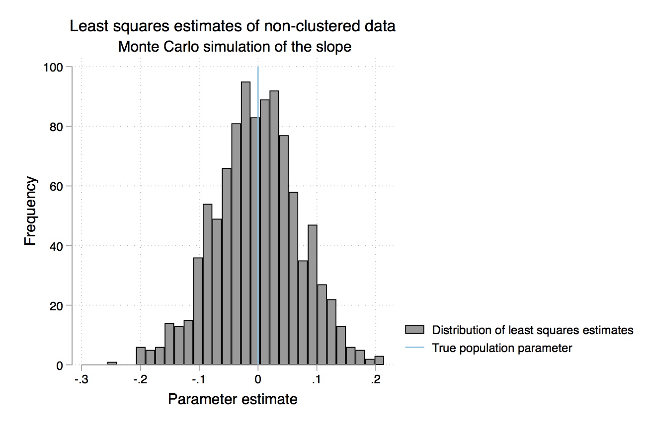
Figure 2.5: Distribution of the least squares estimator over 1,000 random draws.

Setting the significance level at 5%, we should incorrectly reject the null that $\beta_1=0$ about 5% of the time in our simulations. But let’s check the confidence intervals. As can be seen in Figure 2.6, about 95% of the 95% confidence intervals contain the true value of $\beta_1$, which is zero. In words, this means that we incorrectly reject the null about 5% of the time.

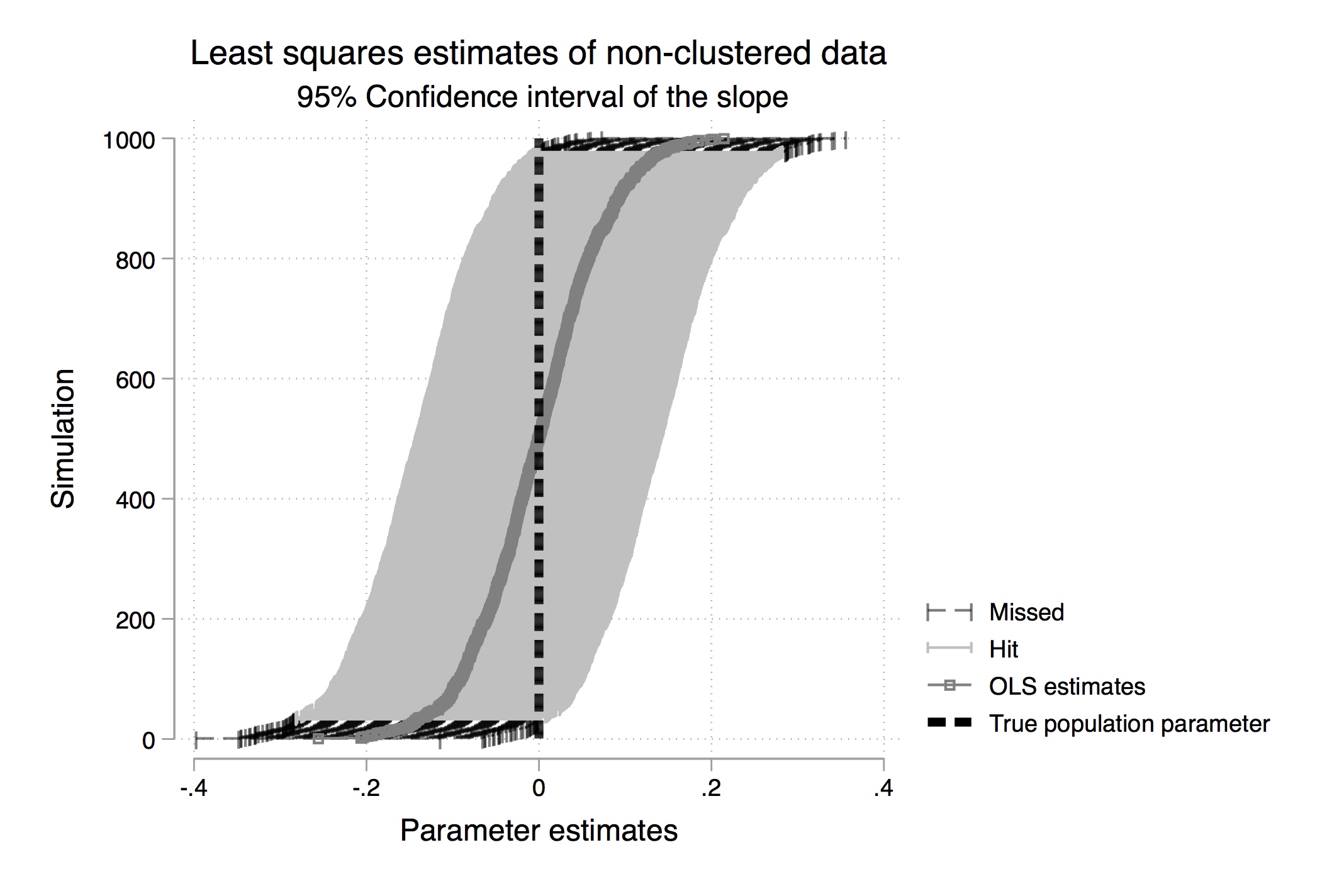
Figure 2.6: Distribution of the 95% confidence intervals with coloring showing those which are incorrectly rejecting the null.

But what happens when we use least squares with clustered data? To see that, let’s resimulate our data with observations that are no longer independent draws in a given cluster of observations.

cluster2.do

Code

clear all
set seed 20140
local n_sims = 1000
set obs `n_sims'

* Create the variables that will contain the results of each simulation
generate beta_0 = .
generate beta_0_l = .
generate beta_0_u = .
generate beta_1 = .
generate beta_1_l = .
generate beta_1_u = .


* Provide the true population parameters
local beta_0_true = 0.4
local beta_1_true = 0
local rho = 0.5

* Simulate a linear regression. Clustered data (x and e are clustered)


quietly {
forvalues i = 1(1) `n_sims' {
    preserve
    clear
    set obs 50
    
    * Generate cluster level data: clustered x and e
    generate int cluster_ID = _n
    generate x_cluster = rnormal(0,1)
    generate e_cluster = rnormal(0, sqrt(`rho'))
    expand 20
    bysort cluster_ID : gen int ind_in_clusterID = _n

    * Generate individual level data
    generate x_individual = rnormal(0,1)
    generate e_individual = rnormal(0,sqrt(1 - `rho'))

    * Generate x and e
    generate x = x_individual + x_cluster
    generate e = e_individual + e_cluster
    generate y = `beta_0_true' + `beta_1_true'*x + e
    
* Least Squares Estimates
    regress y x
    local b0 = _b[_cons]
    local b1 = _b[x]
    local df = e(df_r)
    local critical_value = invt(`df', 0.975)
    * Save the results
    restore
    replace beta_0 = `b0' in `i'
    replace beta_0_l = beta_0 - `critical_value'*_se[_cons]
    replace beta_0_u = beta_0 + `critical_value'*_se[_cons]
    replace beta_1 = `b1' in `i'
    replace beta_1_l = beta_1 - `critical_value'*_se[x]
    replace beta_1_u = beta_1 + `critical_value'*_se[x]
}
}

gen false = (beta_1_l > 0 )
replace false = 2 if beta_1_u < 0
replace false = 3 if false == 0
tab false

* Plot the parameter estimate
hist beta_1, frequency addplot(pci 0 0 100 0) title("Least squares estimates of clustered Data") subtitle(" Monte Carlo simulation of the slope") legend(label(1 "Distribution of least squares estimates") label(2 "True population parameter")) xtitle("Parameter estimate")

cluster2.R

Code

#- Analysis of Clustered Data - part 2
#- Courtesy of Dr. Yuki Yanai, 
#- http://yukiyanai.github.io/teaching/rm1/contents/R/clustered-data-analysis.html

library('arm')
library('mvtnorm')
library('lme4')
library('multiwayvcov')
library('clusterSEs')
library('ggplot2')
library('dplyr')
library('haven')

#Data with clusters
sim_params <- c(.4, 0)   # beta1 = 0: no effect of x on y
sim_cluster_ols <- run_cluster_sim(n_sims = 10000, param = sim_params)
hist_cluster_ols <- hist_nocluster %+% sim_cluster_ols
print(hist_cluster_ols)

cluster2.py

Code

import numpy as np 
import pandas as pd 
import statsmodels.api as sm 
import statsmodels.formula.api as smf 
from itertools import combinations 
import plotnine as p

# read data
import ssl
ssl._create_default_https_context = ssl._create_unverified_context
def read_data(file): 
    return pd.read_stata("https://github.com/scunning1975/mixtape/raw/master/" + file)


def gen_cluster(param = (.1, .5), n = 1000, n_cluster = 50, rho = .5):
    # Function to generate clustered data

    # individual level
    Sigma_i = np.array((1, 0, 0, 1 - rho)).reshape(2,2)

    values_i = np.random.multivariate_normal(np.zeros(2), Sigma_i, size = n)

    # cluster level
    cluster_name = np.repeat(np.arange(1, n_cluster+1), repeats = n / n_cluster)
    Sigma_cl = np.array((1, 0, 0, rho)).reshape(2,2)
    values_cl = np.random.multivariate_normal(np.zeros(2),Sigma_cl, size = n_cluster)

    # predictor var consists of individual- and cluster-level components
    x = values_i[: , 0] + np.repeat(values_cl[: , 0], repeats = n / n_cluster)

    # error consists of individual- and cluster-level components
    error = values_i[: , 1] + np.repeat(values_cl[: , 1], repeats = n / n_cluster)

    # data generating process
    y = param[0] + param[1]*x + error
    
    df = pd.DataFrame({'x':x, 'y':y, 'cluster': cluster_name})
    return df

def cluster_sim(param = (.1, .5), n = 1000, n_cluster = 50,
                        rho = .5, cluster_robust = False):

    df = gen_cluster(param = param, n = n , n_cluster = n_cluster, rho = rho)

    if not cluster_robust:
        fit = sm.OLS.from_formula('y ~ x', data = df).fit()
    else: # cluster-robust SE
        fit = sm.OLS.from_formula('y ~ x', data = df).fit(cov_type='cluster', cov_kwds={'groups': df['cluster']})
    
    b1 = fit.params[1]
    Sigma = fit.cov_params()   
    
    se = np.sqrt(np.diag(Sigma)[1])
    ci95 = se*1.96
    b1_ci95 = (b1-ci95, b1+ci95)

    return (b1, se, *b1_ci95)

def run_cluster_sim(n_sims = 1000, param = (.1, .5), n = 1000,
                            n_cluster = 50, rho = .5, cluster_robust = False):

    res = [cluster_sim(param = param, n = n, rho = rho,
                                      n_cluster = n_cluster,
                                      cluster_robust = cluster_robust) for x in range(n_sims)]
    df = pd.DataFrame(res)
    df.columns = ('b1', 'se_b1', 'ci95_lower', 'ci95_upper')
    df['param_caught'] = (df['ci95_lower'] <= param[1]) & (param[1] <= df['ci95_upper'])
    df['id'] = df.index
    return df


# Simulation clustered SE
sim_params = [.4, 0] # beta1 = 0: no effect of x on y
sim_nocluster = run_cluster_sim(n_sims=1000, param = sim_params, cluster_robust = False)

p.ggplot(sim_nocluster, p.aes('b1')) +  p.geom_histogram(color = 'black') +  p.geom_vline(xintercept = sim_params[1], color = 'red')

1 - sum(sim_nocluster.param_caught)/sim_nocluster.shape[0]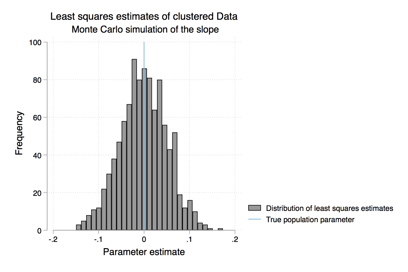

Figure 2.7: Distribution of the least squares estimator over 1,000 random draws.

As can be seen in Figure 2.7, the least squares estimate has a narrower spread than that of the estimates when the data isn’t clustered. But to see this a bit more clearly, let’s look at the confidence intervals again.

cluster3.do

Code

sort beta_1
gen int sim_ID = _n
gen beta_1_True = 0

* Plot of the Confidence Interval
twoway rcap beta_1_l beta_1_u sim_ID if beta_1_l > 0 | beta_1_u < 0  , horizontal lcolor(pink) || || ///
rcap beta_1_l beta_1_u sim_ID if beta_1_l < 0 & beta_1_u > 0 , horizontal ysc(r(0)) || || ///
connected sim_ID beta_1 || || ///
line sim_ID beta_1_True, lpattern(dash) lcolor(black) lwidth(1) ///  
title("Least squares estimates of clustered data") subtitle(" 95% Confidence interval of the slope") ///
legend(label(1 "Missed") label(2 "Hit") label(3 "OLS estimates") label(4 "True population parameter")) xtitle("Parameter estimates") ///
ytitle("Simulation")

cluster3.R

Code

#- Analysis of Clustered Data - part 3
#- Courtesy of Dr. Yuki Yanai, 
#- http://yukiyanai.github.io/teaching/rm1/contents/R/clustered-data-analysis.html

library('arm')
library('mvtnorm')
library('lme4')
library('multiwayvcov')
library('clusterSEs')
library('ggplot2')
library('dplyr')
library('haven')

#Confidence interval
ci95_cluster_ols <- ci95_nocluster %+% sample_n(sim_cluster_ols, 100)
print(ci95_cluster_ols)

sim_cluster_ols %>% summarize(type1_error = 1 - sum(param_caught)/n())

cluster3.py

Code

import numpy as np 
import pandas as pd 
import statsmodels.api as sm 
import statsmodels.formula.api as smf 
from itertools import combinations 
import plotnine as p

# read data
import ssl
ssl._create_default_https_context = ssl._create_unverified_context
def read_data(file): 
    return pd.read_stata("https://github.com/scunning1975/mixtape/raw/master/" + file)


def gen_cluster(param = (.1, .5), n = 1000, n_cluster = 50, rho = .5):
    # Function to generate clustered data

    # individual level
    Sigma_i = np.array((1, 0, 0, 1 - rho)).reshape(2,2)

    values_i = np.random.multivariate_normal(np.zeros(2), Sigma_i, size = n)

    # cluster level
    cluster_name = np.repeat(np.arange(1, n_cluster+1), repeats = n / n_cluster)
    Sigma_cl = np.array((1, 0, 0, rho)).reshape(2,2)
    values_cl = np.random.multivariate_normal(np.zeros(2),Sigma_cl, size = n_cluster)

    # predictor var consists of individual- and cluster-level components
    x = values_i[: , 0] + np.repeat(values_cl[: , 0], repeats = n / n_cluster)

    # error consists of individual- and cluster-level components
    error = values_i[: , 1] + np.repeat(values_cl[: , 1], repeats = n / n_cluster)

    # data generating process
    y = param[0] + param[1]*x + error
    
    df = pd.DataFrame({'x':x, 'y':y, 'cluster': cluster_name})
    return df

def cluster_sim(param = (.1, .5), n = 1000, n_cluster = 50,
                        rho = .5, cluster_robust = False):

    df = gen_cluster(param = param, n = n , n_cluster = n_cluster, rho = rho)

    if not cluster_robust:
        fit = sm.OLS.from_formula('y ~ x', data = df).fit()
    else: # cluster-robust SE
        fit = sm.OLS.from_formula('y ~ x', data = df).fit(cov_type='cluster', cov_kwds={'groups': df['cluster']})
    
    b1 = fit.params[1]
    Sigma = fit.cov_params()   
    
    se = np.sqrt(np.diag(Sigma)[1])
    ci95 = se*1.96
    b1_ci95 = (b1-ci95, b1+ci95)

    return (b1, se, *b1_ci95)

def run_cluster_sim(n_sims = 1000, param = (.1, .5), n = 1000,
                            n_cluster = 50, rho = .5, cluster_robust = False):

    res = [cluster_sim(param = param, n = n, rho = rho,
                                      n_cluster = n_cluster,
                                      cluster_robust = cluster_robust) for x in range(n_sims)]
    df = pd.DataFrame(res)
    df.columns = ('b1', 'se_b1', 'ci95_lower', 'ci95_upper')
    df['param_caught'] = (df['ci95_lower'] <= param[1]) & (param[1] <= df['ci95_upper'])
    df['id'] = df.index
    return df


# Simulation clustered SE
sim_params = [.4, 0] # beta1 = 0: no effect of x on y
sim_nocluster = run_cluster_sim(n_sims=1000, param = sim_params, cluster_robust = False)


p.ggplot(sim_nocluster.sample(100).sort_values('b1'),
                         p.aes(x = 'factor(id)', y = 'b1', 
                             ymin = 'ci95_lower', ymax = 'ci95_upper',
                             color = 'param_caught')) +\
  p.geom_hline(yintercept = sim_params[1], linetype = 'dashed') +\
  p.geom_pointrange() +\
  p.labs(x = 'sim ID', y = 'b1', title = 'Randomly Chosen 100 95% CIs') +\
  p.scale_color_discrete(name = 'True param value', labels = ('missed', 'hit')) +\
  p.coord_flip()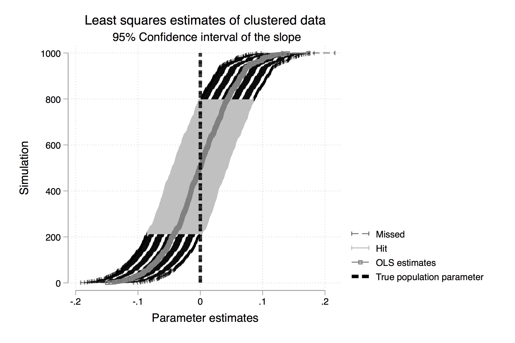

Figure 2.8: Distribution of 1,000 95% confidence intervals with dashed region representing those estimates that incorrectly reject the null.

Figure 2.8 shows the distribution of 95% confidence intervals from the least squares estimates. As can be seen, a much larger number of estimates incorrectly rejected the null hypothesis when the data was clustered. The standard deviation of the estimator shrinks under clustered data, causing us to reject the null incorrectly too often. So what can we do?

cluster4.do

Code

* Robust Estimates
clear all
local n_sims = 1000
set obs `n_sims'

* Create the variables that will contain the results of each simulation
generate beta_0_robust = .
generate beta_0_l_robust = .
generate beta_0_u_robust = .
generate beta_1_robust = .
generate beta_1_l_robust = .
generate beta_1_u_robust = .

* Provide the true population parameters
local beta_0_true = 0.4
local beta_1_true = 0
local rho = 0.5

quietly {
forvalues i = 1(1) `n_sims' {
    preserve
    clear
    set obs 50
    
    * Generate cluster level data: clustered x and e
    generate int cluster_ID = _n
    generate x_cluster = rnormal(0,1)
    generate e_cluster = rnormal(0, sqrt(`rho'))
    expand 20
    bysort cluster_ID : gen int ind_in_clusterID = _n

    * Generate individual level data
    generate x_individual = rnormal(0,1)
    generate e_individual = rnormal(0,sqrt(1 - `rho'))

    * Generate x and e
    generate x = x_individual + x_cluster
    generate e = e_individual + e_cluster
    generate y = `beta_0_true' + `beta_1_true'*x + e
    regress y x, cl(cluster_ID)
    local b0_robust = _b[_cons]
    local b1_robust = _b[x]
    local df = e(df_r)
    local critical_value = invt(`df', 0.975)
    * Save the results
    restore
    replace beta_0_robust = `b0_robust' in `i'
    replace beta_0_l_robust = beta_0_robust - `critical_value'*_se[_cons]
    replace beta_0_u_robust = beta_0_robust + `critical_value'*_se[_cons]
    replace beta_1_robust = `b1_robust' in `i'
    replace beta_1_l_robust = beta_1_robust - `critical_value'*_se[x]
    replace beta_1_u_robust = beta_1_robust + `critical_value'*_se[x]

}
}

* Plot the histogram of the parameters estimates of the robust least squares
gen false = (beta_1_l_robust > 0 )
replace false = 2 if beta_1_u_robust < 0
replace false = 3 if false == 0
tab false

* Plot the parameter estimate
hist beta_1_robust, frequency addplot(pci 0 0 110 0) title("Robust least squares estimates of clustered data") subtitle(" Monte Carlo simulation of the slope") legend(label(1 "Distribution of robust least squares estimates") label(2 "True population parameter")) xtitle("Parameter estimate")

sort beta_1_robust
gen int sim_ID = _n
gen beta_1_True = 0

* Plot of the Confidence Interval
twoway rcap beta_1_l_robust beta_1_u_robust sim_ID if beta_1_l_robust > 0 | beta_1_u_robust < 0, horizontal lcolor(pink) || || rcap beta_1_l_robust beta_1_u_robust sim_ID if beta_1_l_robust < 0 & beta_1_u_robust > 0 , horizontal ysc(r(0)) || || connected sim_ID beta_1_robust || || line sim_ID beta_1_True, lpattern(dash) lcolor(black) lwidth(1) title("Robust least squares estimates of clustered data") subtitle(" 95% Confidence interval of the slope") legend(label(1 "Missed") label(2 "Hit") label(3 "Robust estimates") label(4 "True population parameter")) xtitle("Parameter estimates") ytitle("Simulation")

cluster4.R

Code

#- Analysis of Clustered Data - part 4
#- Courtesy of Dr. Yuki Yanai, 
#- http://yukiyanai.github.io/teaching/rm1/contents/R/clustered-data-analysis.html

library('arm')
library('mvtnorm')
library('lme4')
library('multiwayvcov')
library('clusterSEs')
library('ggplot2')
library('dplyr')
library('haven')

#clustered robust
sim_params <- c(.4, 0)   # beta1 = 0: no effect of x on y
sim_cluster_robust <- run_cluster_sim(n_sims = 10000, param = sim_params,
                                      cluster_robust = TRUE)

hist_cluster_robust <- hist_nocluster %+% sim_cluster_ols
print(hist_cluster_robust)

#Confidence Intervals
ci95_cluster_robust <- ci95_nocluster %+% sample_n(sim_cluster_robust, 100)
print(ci95_cluster_robust)

sim_cluster_robust %>% summarize(type1_error = 1 - sum(param_caught)/n())

cluster4.py

Code

import numpy as np 
import pandas as pd 
import statsmodels.api as sm 
import statsmodels.formula.api as smf 
from itertools import combinations 
import plotnine as p

# read data
import ssl
ssl._create_default_https_context = ssl._create_unverified_context
def read_data(file): 
    return pd.read_stata("https://github.com/scunning1975/mixtape/raw/master/" + file)



def gen_cluster(param = (.1, .5), n = 1000, n_cluster = 50, rho = .5):
    # Function to generate clustered data

    # individual level
    Sigma_i = np.array((1, 0, 0, 1 - rho)).reshape(2,2)

    values_i = np.random.multivariate_normal(np.zeros(2), Sigma_i, size = n)

    # cluster level
    cluster_name = np.repeat(np.arange(1, n_cluster+1), repeats = n / n_cluster)
    Sigma_cl = np.array((1, 0, 0, rho)).reshape(2,2)
    values_cl = np.random.multivariate_normal(np.zeros(2),Sigma_cl, size = n_cluster)

    # predictor var consists of individual- and cluster-level components
    x = values_i[: , 0] + np.repeat(values_cl[: , 0], repeats = n / n_cluster)

    # error consists of individual- and cluster-level components
    error = values_i[: , 1] + np.repeat(values_cl[: , 1], repeats = n / n_cluster)

    # data generating process
    y = param[0] + param[1]*x + error
    
    df = pd.DataFrame({'x':x, 'y':y, 'cluster': cluster_name})
    return df

def cluster_sim(param = (.1, .5), n = 1000, n_cluster = 50,
                        rho = .5, cluster_robust = False):

    df = gen_cluster(param = param, n = n , n_cluster = n_cluster, rho = rho)

    if not cluster_robust:
        fit = sm.OLS.from_formula('y ~ x', data = df).fit()
    else: # cluster-robust SE
        fit = sm.OLS.from_formula('y ~ x', data = df).fit(cov_type='cluster', cov_kwds={'groups': df['cluster']})
    
    b1 = fit.params[1]
    Sigma = fit.cov_params()   
    
    se = np.sqrt(np.diag(Sigma)[1])
    ci95 = se*1.96
    b1_ci95 = (b1-ci95, b1+ci95)

    return (b1, se, *b1_ci95)


def run_cluster_sim(n_sims = 1000, param = (.1, .5), n = 1000,
                            n_cluster = 50, rho = .5, cluster_robust = False):

    res = [cluster_sim(param = param, n = n, rho = rho,
                                      n_cluster = n_cluster,
                                      cluster_robust = cluster_robust) for x in range(n_sims)]
    df = pd.DataFrame(res)
    df.columns = ('b1', 'se_b1', 'ci95_lower', 'ci95_upper')
    df['param_caught'] = (df['ci95_lower'] <= param[1]) & (param[1] <= df['ci95_upper'])
    df['id'] = df.index
    return df


# Simulation clustered SE
sim_params = [.4, 0] # beta1 = 0: no effect of x on y
sim_nocluster = run_cluster_sim(n_sims=1000, param = sim_params, cluster_robust = True)

p.ggplot(sim_nocluster, p.aes('b1')) +  p.geom_histogram(color = 'black') +  p.geom_vline(xintercept = sim_params[1], color = 'red')

p.ggplot(sim_nocluster.sample(100).sort_values('b1'),
                         p.aes(x = 'factor(id)', y = 'b1', 
                             ymin = 'ci95_lower', ymax = 'ci95_upper',
                             color = 'param_caught')) +\
  p.geom_hline(yintercept = sim_params[1], linetype = 'dashed') +\
  p.geom_pointrange() +\
  p.labs(x = 'sim ID', y = 'b1', title = 'Randomly Chosen 100 95% CIs') +\
  p.scale_color_discrete(name = 'True param value', labels = ('missed', 'hit')) +\
  p.coord_flip()


1 - sum(sim_nocluster.param_caught)/sim_nocluster.shape[0]

Now in this case, notice that we included the “, cluster(cluster_ID)” syntax in our regression command. Before we dive in to what this syntax did, let’s look at how the confidence intervals changed. Figure 2.9 shows the distribution of the 95% confidence intervals where, again, the darkest region represents those estimates that incorrectly rejected the null. Now, when there are observations whose errors are correlated within a cluster, we find that estimating the model using least squares leads us back to a situation in which the type I error has decreased considerably.

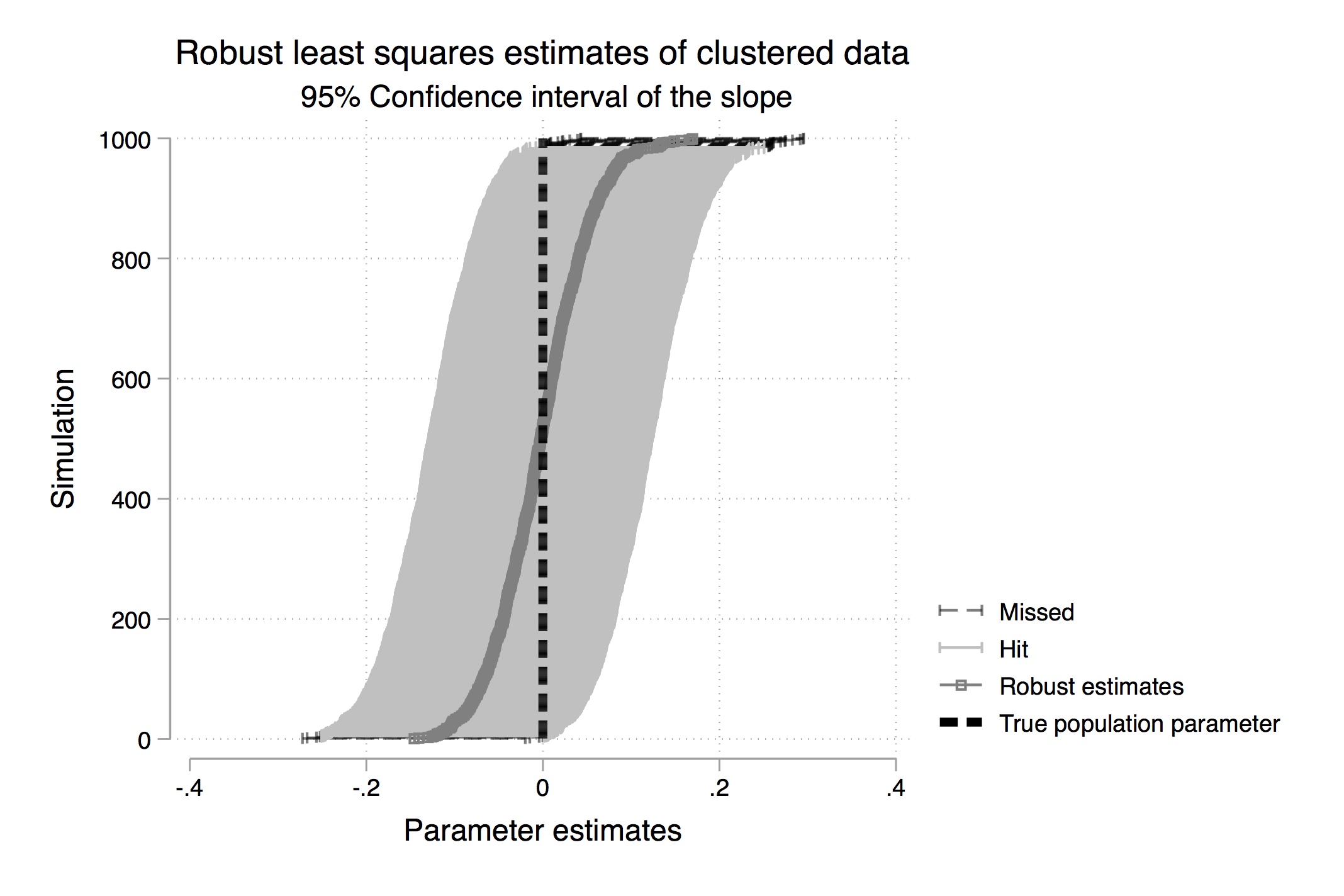
Figure 2.9: Distribution of 1,000 95% confidence intervals from a cluster robust least squares regression with dashed region representing those estimates that incorrectly reject the null.

This leads us to a natural question: what did the adjustment of the estimator’s variance do that caused the type I error to decrease by so much? Whatever it’s doing, it sure seems to be working! Let’s dive in to this adjustment with an example. Consider the following model: \[ y_{ig}=x_{ig}'\beta+u_{ig}\quad \text{where } $g \in 1, \dots, G$ \] and \[ E[u_{ig}u_{jg'}'] \] which equals zero if $g=g'$ and equals $\sigma_{(ij)g}$ if $g\ne g'$.

Let’s stack the data by cluster first. \[ y_g=x_g' \beta+u_g \] The OLS estimator is still $\widehat{\beta}= E[X'X]^{-1}X'Y$. We just stacked the data, which doesn’t affect the estimator itself. But it does change the variance. \[ V(\beta)=E\Big[[X'X]^{-1}X' \Omega X[X'X]^{-1}\Big] \] With this in mind, we can now write the variance-covariance matrix for clustered data as \[ \widehat{V}(\widehat{\beta})=[X'X]^{-1} \left[ \sum_{i=1}^G x'_g \widehat{u}_g \widehat{u}_g'\right][X'X]^{-1} \]

Adjusting for clustered data will be quite common in your applied work given the ubiquity of clustered data in the first place. It’s absolutely essential for working in the panel contexts, or in repeated cross-sections like the difference-in-differences design. But it also turns out to be important for experimental design, because often, the treatment will be at a higher level of aggregation than the microdata itself. In the real world, though, you can never assume that errors are independent draws from the same distribution. You need to know how your variables were constructed in the first place in order to choose the correct error structure for calculating your standard errors. If you have aggregate variables, like class size, then you’ll need to cluster at that level. If some treatment occurred at the state level, then you’ll need to cluster at that level. There’s a large literature available that looks at even more complex error structures, such as multi-way clustering (Cameron, Gelbach, and Miller 2011).

But even the concept of the sample as the basis of standard errors may be shifting. It’s becoming increasingly less the case that researchers work with random samples; they are more likely working with administrative data containing the population itself, and thus the concept of sampling uncertainty becomes strained.²⁸ For instance, Manski and Pepper (2018) wrote that “random sampling assumptions …are not natural when considering states or counties as units of observation.” So although a metaphor of a superpopulation may be useful for extending these classical uncertainty concepts, the ubiquity of digitized administrative data sets has led econometricians and statisticians to think about uncertainty in other ways.

New work by Abadie et al. (2020) explores how sampling-based concepts of the standard error may not be the right way to think about uncertainty in the context of causal inference, or what they call design-based uncertainty. This work in many ways anticipates the next two chapters because of its direct reference to the concept of the counterfactual. Design-based uncertainty is a reflection of not knowing which values would have occurred had some intervention been different in counterfactual. And Abadie et al. (2020) derive standard errors for design-based uncertainty, as opposed to sampling-based uncertainty. As luck would have it, those standard errors are usually smaller.

Let’s now move into these fundamental concepts of causality used in applied work and try to develop the tools to understand how counterfactuals and causality work together.

Causal Inference:
The Mixtape.

Buy the print version today:

Buy from Amazon Buy from Yale Press

Abadie, Alberto, Susan Athey, Guido W. Imbens, and Jeffrey M. Wooldridge. 2020. “Sampling-Based Versus Design-Based Uncertainty in Regression Analysis.” Econometrica 88 (0): 265–96.

Angrist, Joshua D., and Jorn-Steffen Pischke. 2009. Mostly Harmless Econometrics. 1st ed. Princeton University Press.

Cameron, A. Colin, Jonah B. Gelbach, and Douglas L. Miller. 2011. “Robust Inference with Multiway Clustering.” Journal of Business and Economic Statistics 29 (2): 238–49.

Filoso, Valerio. 2013. “Regression Anatomy, Revealed.” The Stata Journal 13 (1): 92–106. https://doi.org/10.1177/1536867X1301300107.

Frisch, Ragnar, and Frederick V. Waugh. 1933. “Partial Time Regressions as Compared with Individuals Trends.” Econometrica 1 (4): 387–401.

Holtzman, Wayne H. 1950. “The Unbiased Estimate of the Population Variance and Standard Deviation.” The American Journal of Psychology 63 (4): 615–17.

Lovell, Michael C. 1963. “Seasonal Adjustment of Economic Time Series and Multiple Regression Analysis.” Journal of the American Statistical Association 58 (304): 991–1010.

———. 2008. “A Simple Proof of the FWL Theorem.” Journal of Economic Education 39 (1): 88–91.

Manski, Charles F., and John V. Pepper. 2018. “How Do Right-to-Carry Laws Affect Crime Rates? Coping with Ambiguity Using Bounded-Variation Assumptions.” Review of Economics and Statistics 100 (2): 232–44.

Mcgrayne, Sharon Bertsch. 2012. The Theory That Would Not Die: How Bayes’ Rule Cracked the Enigma Code, Hunted down Russian Submarines, and Emerged Triumphant from Two Centuries of Controversy. Yale University Press.

White, Halbert. 1980. “A Heteroskedasticity-Consistent Covariance Matrix Estimator and a Direct Test for Heteroskedasticity.” Econometrica 48 (4): 817–38.

Wooldridge, Jeffrey. 2010. Econometric Analysis of Cross Section and Panel Data. 2nd ed. MIT Press.

———. 2015. Introductory Econometrics: A Modern Approach. 6th ed. South-Western College Pub.

The probability rolling a 5 using one six-sided die is $\dfrac{1}{6}=0.167$.↩︎
The set notation $\cup$ means “union” and refers to two events occurring together.↩︎
Why are they different? Because 0.83 is an approximation of $\Pr(B\mid A)$, which was technically 0.833…trailing.↩︎
There’s an ironic story in which someone posed the Monty Hall question to the columnist, Marilyn vos Savant. Vos Savant had an extremely high IQ and so people would send in puzzles to stump her. Without the Bayesian decomposition, using only logic, she got the answer right. Her column enraged people, though. Critics wrote in to mansplain how wrong she was, but in fact it was they who were wrong.↩︎
For a more complete review of regression, see Wooldridge (2010) and Wooldridge (2015). I stand on the shoulders of giants.↩︎
The law of total probability requires that all marginal probabilities sum to unity.↩︎
Whenever possible, I try to use the “hat” to represent an estimated statistic. Hence $\widehat{S}^2$ instead of just $S^2$. But it is probably more common to see the sample variance represented as $S^2$.↩︎
This is not necessarily causal language. We are speaking first and generally in terms of two random variables systematically moving together in some measurable way.↩︎
Notice that the conditional expectation passed through the linear function leaving a constant, because of the first property of the expectation operator, and a constant times $x$. This is because the conditional expectation of $E[X\mid X]=X$. This leaves us with $E[u\mid X]$ which under zero conditional mean is equal to 0.↩︎
Notice that we are dividing by $n$, not $n-1$. There is no degrees-of-freedom correction, in other words, when using samples to calculate means. There is a degrees-of-freedom correction when we start calculating higher moments.↩︎
Recall from much earlier that: \[\begin{align} \sum_{i=1}^n (x_i -\overline{x})(y_i-\overline{y}) & = \sum_{i=1}^n x_i(y_i-\overline{y}) \\ & =\sum_{i=1}^n(x_i-\overline{x})y_i \\ & =\sum_{i=1}^n x_iy_i-n(\overline{x}\overline{y}) \end{align}\]↩︎
It isn’t exactly 0 even though $u$ and $x$ are independent. Think of it as $u$ and $x$ are independent in the population, but not in the sample. This is because sample characteristics tend to be slightly different from population properties due to sampling error.↩︎
Using the Stata code from Table 2.6, you can show these algebraic properties yourself. I encourage you to do so by creating new variables equaling the product of these terms and collapsing as we did with the other variables. That sort of exercise may help convince you that the aforementioned algebraic properties always hold.↩︎
Recall the earlier discussion about degrees-of-freedom correction.↩︎
This section is a review of traditional econometrics pedagogy. We cover it for the sake of completeness. Traditionally, econometricians motivated their discuss of causality through ideas like unbiasedness and consistency.↩︎
Told you we would use this result a lot.↩︎
I find it interesting that we see so many $\dfrac{cov}{var}$ terms when working with regres-
sion. They show up constantly. Keep your eyes peeled.↩︎
The standard error I found from running this on one sample of data was 0.0403616.↩︎
I highly encourage the interested reader to study Angrist and Pischke (2009), who have an excellent discussion of LIE there.↩︎
Let’s take a concrete example of this proof. Let $h(x_i)=\alpha+\gamma x_i$. Then take the joint expectation $E(h(x_i)\varepsilon_i)=E([\alpha+\gamma x_i] \varepsilon_i)$. Then take conditional expectations $E (\alpha\mid x_i )+E(\gamma\mid x_i) E(x_i\mid x_i)E(\varepsilon\mid x_i)\}=\alpha+ x_iE(\varepsilon_i\mid x_i)=0$ after we pass the conditional expectation through.↩︎
See Angrist and Pischke (2009) for a proof.↩︎
A helpful proof of the Frisch-Waugh-Lovell theorem can be found in Lovell (2008).↩︎
While randomly having kids may sound fun, I encourage you to have kids when you want to have them. Contact your local high school health teacher to learn more about a number of methods that can reasonably minimize the number of random children you create.↩︎
Almost certainly a ridiculous assumption, but stick with me.↩︎
There does exist an unbiased estimator of $\sigma$, but it’s tedious and hardly anyone in economics seems to use it. See Holtzman (1950).↩︎
No one even bothers to cite White (1980) anymore, just like how no one cites Leibniz or Newton when using calculus. Eicker, Huber, and White created a solution so valuable that it got separated from the original papers when it was absorbed into the statistical toolkit.↩︎
Hat tip to Ben Chidmi, who helped create this simulation in Stata.↩︎
Usually we appeal to superpopulations in such situations where the observed population is simply itself a draw from some “super” population.↩︎

Event labels	Coach is not rehired \((\sim B)\)	Coach is rehired \((B)\)	Total
\((A)\) Bowl game	\(\Pr(A,\sim B)\)=0.1	\(\Pr(A,B)\)=0.5	\(\Pr(A)\)=0.6
\((\sim A)\) no Bowl game	\(\Pr(\sim A, \sim B)=0.1\)	\(\Pr(\sim A,B)=0.3\)	\(\Pr(\sim A)=0.4\)
Total	\(\Pr(\sim B)=0.2\)	\(\Pr(B)=0.8\)	1.0

\(x\)	\(x-\overline{x}\)
10	2
4	\(-4\)
13	5
5	\(-3\)
Mean=8	Sum=0

no.	\(x\)	\(u\)	\(y\)	\(\widehat{y}\)	\(\widehat{u}\)	\(x\widehat{u}\)	\(\widehat{y}\widehat{u}\)
1.	\(-4.381653\)	\(-32.95803\)	\(-38.72134\)	\(-3.256034\)	\(-35.46531\)	155.3967	115.4762
2.	\(-13.28403\)	\(-8.028061\)	\(-31.59613\)	\(-26.30994\)	\(-5.28619\)	70.22192	139.0793
3.	\(-.0982034\)	17.80379	20.60738	7.836532	12.77085	\(-1.254141\)	100.0792
4.	\(-.1238423\)	\(-9.443188\)	\(-6.690872\)	7.770137	\(-14.46101\)	1.790884	\(-112.364\)
5.	4.640209	13.18046	25.46088	20.10728	5.353592	24.84179	107.6462
6.	\(-1.252096\)	\(-34.64874\)	\(-34.15294\)	4.848374	\(-39.00131\)	48.83337	\(-189.0929\)
7.	11.58586	9.118524	35.29023	38.09396	\(-2.80373\)	\(-32.48362\)	\(-106.8052\)
8.	\(-5.289957\)	82.23296	74.65305	\(-5.608207\)	80.26126	\(-424.5786\)	\(-450.1217\)
9.	\(-.2754041\)	11.60571	14.0549	7.377647	6.677258	\(-1.838944\)	49.26245
10.	\(-19.77159\)	\(-14.61257\)	\(-51.15575\)	\(-43.11034\)	\(-8.045414\)	159.0706	346.8405
Sum	\(-28.25072\)	34.25085	7.749418	7.749418	1.91e-06	\(-6.56e-06\)	.0000305

Causal Inference: The Mixtape.

2.1 Basic probability theory

2.2 Events and conditional probability

2.3 Probability tree

2.4 Venn diagrams and sets

2.5 Contingency tables

2.6 Monty Hall example

2.7 Summation operator

2.8 Expected value

2.9 Variance

2.10 Covariance

2.11 Population model

2.12 Mean independence

Causal Inference: The Mixtape.

2.13 Ordinary least squares

2.14 Algebraic Properties of OLS

2.15 Goodness-of-fit

2.16 Expected value of OLS

2.17 Law of iterated expectations

2.18 CEF decomposition property

2.19 CEF prediction property

2.20 ANOVA theory

2.21 Linear CEF theorem

2.22 Best linear predictor theorem

2.23 Regression CEF theorem

2.24 Regression anatomy theorem

2.25 Variance of the OLS estimators

2.26 Robust standard errors

2.27 Cluster robust standard errors

Causal Inference: The Mixtape.

Causal Inference:
The Mixtape.

Causal Inference:
The Mixtape.

Causal Inference:
The Mixtape.