3  Directed Acyclic Graphs

The history of graphical causal modeling goes back to the early 20th century with Sewell Wright, one of the fathers of modern genetics and son of economist Philip Wright. Sewell developed path diagrams for genetics, and Philip, we believe, adapted them for econometric identification (Matsueda 2012).¹ But despite its early adoption, graphical modeling for causal inference was largely ignored by economists with only a few exceptions (Heckman and Pinto 2015; Imbens 2020).

Today, the person most often associated with graphical models is the computer scientist Judea Pearl. Pearl developed a general theory of causal inference that expounds on the usefulness of the directed graph notation in his magnum opus Pearl (2009). Since I think graphical models are immensely helpful for designing a credible identification strategy, I have chosen to include these models for your consideration. This chapter will only function as a simple introduction of graphical models, as we will be selective in the book about its use, but I highly encourage you to read Morgan and Winship (2014) and Pearl, Glymour, and Jewell (2016) if you are wishing to build on this material.

3.1 Introduction to DAG Notation

Directed acyclic graphs (DAGs) offer a powerful visual framework for representing and reasoning about causal relationships. At their core, DAGs capture the directional flow of causality—each arrow represents an immediate cause-and-effect relationship between variables, and the absence of cycles reflects the unidirectional nature of time and causation. While social science theories often allow for reverse causality or feedback loops, DAGs require breaking these cycles into sequential events, making causality more explicit and analyzable.

Despite their simplicity, DAGs are grounded in the same counterfactual framework that underpins potential outcomes. A causal effect is still defined as a comparison between two states of the world: the observed outcome under one intervention and the counterfactual outcome under another. This connection makes DAGs a natural complement to potential outcomes by offering a graphical representation of various assumptions we must make when identifying effects. In fact, this is precisely one of the strengths of this approach — it forces the researcher to think long and hard about the treatment assignment mechanisms, which are one of the main factors that dictate whether one research design is more suitable than another.

In a DAG, nodes represent variables generated by an underlying data-generating process (DGP), and arrows represent causal effects. For example, a direct causal effect is shown as \(D \rightarrow Y\), while mediated effects involve intermediate variables, such as \(D \rightarrow M \rightarrow Y\). An arrow indicates a causal relationship, while the absence of an arrow asserts the lack of one—a critical assumption that must be justified.

But where do DAGs come from? This might be the most important question. A DAG is a theoretical model built from prior knowledge: your field’s theories, empirical studies, expert input, and intuition. It’s not just a broad theory; it’s a theory tailored to your specific data, capturing the world as your data reflects it. For instance, it’s less a general theory of disease and more a theory of disease in a specific place and time, involving particular communities. Writing out a DAG requires more than understanding general principles; it demands an effort to map the causal structure of the specific context your data describes. DAGs distill this knowledge into explicit, credible assumptions, which in turn guide causal inference. These assumptions help identify which methods are most appropriate for estimating causal effects.

I’ve included DAGs in this book because they highlight the critical role of prior knowledge in identifying causal effects. They’re also an intuitive tool for communicating research designs, particularly for complex methods like instrumental variables. Additionally, tools like the backdoor criterion and collider bias make DAGs practical for selecting covariates under unconfoundedness or in difference-in-differences settings. Finally, DAGs provide a common language that bridges structural and reduced-form approaches while reinforcing the idea that assumptions are essential for causal identification (Wolpin 2013).

In the sections ahead, we’ll see how DAGs clarify assumptions in causal inference, help avoid pitfalls like collider bias, and guide effective research design. By the end of this chapter, you’ll be equipped to construct, interpret, and apply DAGs in your own work.

Introducing and Analyzing a Simple DAG

Let’s begin with a simple DAG to illustrate a few basic ideas. I will expand on it to build slightly more complex ones later.

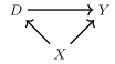
In this DAG, we have three random variables: \(X\), \(D\), and \(Y\). There is a direct path from \(D\) to \(Y\), which represents a causal effect. It is represented by \(D \rightarrow Y\). But there is also a second path from \(D\) to \(Y\) called the backdoor path. The backdoor path is \(D \leftarrow X \rightarrow Y\). While the direct path is a causal effect, the backdoor path is not causal. Rather, it is a process that creates spurious correlations between \(D\) and \(Y\) driven solely by fluctuations in the \(X\) random variable.

The idea of the backdoor path is one of the most important things that we learn from the DAG. It is similar to the notion of omitted variable bias in that it represents a variable, which determines the outcome and the treatment variable. Just as not controlling for a variable like that in a regression creates omitted variable bias, leaving a backdoor open creates bias. The backdoor path is \(D \leftarrow X \rightarrow\) Y. We therefore call \(X\) a confounder in the sense that because it jointly determines \(D\) and \(Y\), it confounds our ability to discern the effect of \(D\) on \(Y\) in naive comparisons.

Think of the backdoor path like this: sometimes when \(D\) takes on different values, \(Y\) takes on different values because \(D\) causes \(Y\). But sometimes \(D\) and \(Y\) take on different values because \(X\) takes on different values, and that bit of the correlation between \(D\) and \(Y\) is purely spurious. The existence of two causal pathways is contained within correlation between \(D\) and \(Y\).

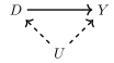
Let’s look at a second DAG, which is subtly different from the first. In the previous example, \(X\) was observed. We know it was observed because the direct edges from \(X\) to \(D\) and \(Y\) were solid lines. But sometimes there exists a confounder that is unobserved, and when there is, we represent its direct edges with dashed lines. Consider the following DAG: Same as before, \(U\) is a noncollider along the backdoor path from \(D\) to \(Y\), but unlike before, \(U\) is unobserved to the researcher.

It exists, but it may simply be missing from the dataset. In this situation, there are two pathways from \(D\) to \(Y\). There’s the direct pathway, \(D \rightarrow Y\), which is the causal effect, and there’s the backdoor pathway \(D \leftarrow U \rightarrow Y\). And since \(U\) is unobserved, that backdoor pathway is open.

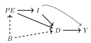
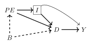
Let’s now move to another example, one that is slightly more realistic. A classical question in labor economics is whether college education increases earnings. According to the Becker human capital model (Becker 1994), education increases one’s marginal product, and since workers are paid their marginal product in competitive markets, education also increases their earnings. But, college education is not random; it is optimally chosen given subjective preferences and resource constraints. We will represent that with the following DAG. As always, let \(D\) be the treatment (e.g., college education) and \(Y\) be the outcome of interest (e.g., earnings). Furthermore, let \(PE\) be parental education, \(I\) be family income, and \(B\) be unobserved background factors, such as genetics, family environment, mental ability, etc.

This DAG is telling a story. And one of the things I like about DAGs is that they invite everyone to listen to the story together. Here is my interpretation of the story being told. Each person has some background. It’s not contained in most datasets, as it measures things like intelligence, contentiousness, mood stability, motivation, family dynamics, and other environmental factors—hence it is unobserved in the picture. Those environmental factors are likely correlated between parent and child, and therefore are subsumed in the variable \(B\).

Background causes a child’s parent to choose her own optimal level of education, and that choice also causes the child to choose their level of education through a variety of channels. First, there is the shared background factors, \(B\). Those background factors cause the child to herself choose a level of education, just as they had with the parent. Second, there’s a direct effect, perhaps through simple modeling of achievement or setting expectations, a kind of peer effect. And third, there’s the effect that parental education has on family earnings, \(I\), which in turn affects how much schooling the child receives. Family earnings may itself affect earnings through bequests and other transfers, as well as external investments in the child’s productivity.

This is a simple story to tell, and the DAG tells it well, but I want to alert your attention to some subtle points contained in this DAG. The DAG is actually telling two stories. It is telling what is happening, and it is telling what is not happening. For instance, notice that \(B\) has no direct effect on the child’s earnings except through its effect on schooling. Is this realistic, though? Economists have long maintained that unobserved ability both determines how much schooling a child gets and also directly affects their earnings, insofar as intelligence and motivation can influence careers. But in this DAG, there is no relationship between background and earnings, which is itself an assumption. And you are free to call foul on this assumption if you think that background factors affect both schooling and the child’s own productivity, which itself should affect wages. So what if you feel there should be an arrow from \(B\) to \(Y\)? Then you would draw one and rewrite all the backdoor paths between \(D\) and \(Y\).

Now that we have a DAG, what do we do? I like to list out all direct and indirect paths (i.e., backdoor paths) between \(D\) and \(Y\). Once I have all those, I have a better sense of where my problems are.

1. Main causal path of interest

   1. \(D \rightarrow Y\) (the causal effect of education on earnings)

2. Backdoor paths

   1. \(D \leftarrow I \rightarrow Y\) (backdoor path # 1)

   2. \(D \leftarrow PE \rightarrow I \rightarrow Y\) (backdoor path #

   3. \(D \leftarrow B \rightarrow PE \rightarrow I \rightarrow Y\) (backdoor path # 3)

So there are four paths between \(D\) and \(Y\): one direct causal effect (schooling’s effect on earnings) and three backdoor paths. These backdoor paths create selection bias when comparing college educated to non-college educated workers’ earnings. If they did not exist, or if they could somehow be closed, then association in earnings between the college and non-college educated workers would be an estimate of college’s effect on earnings, but without such a thing, the SDO would be biased.

But there is one situation in which a backdoor path can actually be blocked, and that is when the variable along that path is something called a collider, which I’ll discuss next.

Colliding

The word “collider” is no doubt a strange one. It does not have an obvious counterpart within statistics or econometrics. So, since it’s novel to many readers, I will go in steps. First, I want to simply show it to you graphically so that you understand how to visualize it. Then later, with a few simulations, I will explain why leaving these variables alone is so crucial in causal inference. Pay careful attention to the direction of the arrows, which have changed in this new drawing of our previous DAG:

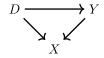
Notice that the arrows this time point to \(X\), rather than away from \(X\) as they had when \(X\) was a confounder. Let’s do like last time, and list all paths from \(D\) to \(Y\).

1. Main causal path of interest

   1. \(D \rightarrow Y\) (causal effect of \(D\) on \(Y\))

2. Backdoor paths

   1. \(D \rightarrow X \leftarrow Y\) (backdoor path # 1)

Just like last time, there are two ways to get from \(D\) to \(Y\). You can get from \(D\) to \(Y\) using the direct (causal) path, \(D \rightarrow Y\). Or you can use the backdoor path, \(D \rightarrow X \leftarrow Y\). But something is different about this backdoor path; do you see it? This time the \(X\) has two arrows pointing to it, not away from it. When two variables cause a third variable along some path, we call that third variable a “collider.” Put differently, \(X\) is a collider along this backdoor path because \(D\) and \(Y\)’s causal effects collide at \(X\).

Colliders are special because when left out as controls, they block backdoor paths between the treatment and the outcome. But their danger is related to that power, too, because when you estimate a model and condition on a collider, it opens up spurious correlations between the treatment and outcome accessible via that now open backdoor path. And since our goal is to eliminate spurious correlations, controlling for colliders is dangerous for their ability to bias our estimates.

3.2 Backdoor Criterion

When our goal is to estimate the main causal path of interest, then we must ensure that all of the backdoor paths are closed. And they are closed in one of two ways: either the noncolliders on that path are controlled for—something called “blocking”—or a collider is on that path, which automatically blocks it for us. When all backdoor paths are closed, then our estimation strategy has successfully satisfied the backdoor criterion, and to understand that, we need to now understand blocking.

Blocking

Satisfying the backdoor criterion means that your estimation strategy has closed all the backdoor paths by both controlling for noncolliders and leaving alone the noncolliders. When such is the case, then the only interpretation of the remaining correlation between the treatment and the outcome is that it’s causal. Let’s review our human capital DAG involving college education, family income, parental education, background, and earnings and use it to illustrate this concept.

Figure 3.1: Simple human capital DAG.

And let’s write down again both the main causal path of interest as well as all the backdoor paths between the treatment and the outcome.

1. Main causal path of interest

   1. \(D \rightarrow Y\) (the causal effect of education on earnings)

2. Backdoor paths

   1. \(D \leftarrow I \rightarrow Y\) (backdoor path # 1)

   2. \(D \leftarrow PE \rightarrow I \rightarrow Y\) (backdoor path #

   3. \(D \leftarrow B \rightarrow PE \rightarrow I \rightarrow Y\) (backdoor path # 3)

In order to identify the effect of \(D\) on \(Y\), we must close all three backdoor paths. On the first backdoor path, only one variable appears (\(I\)) and it is a noncollider. On the second, two variables appear (\(PE\) and \(I\)) and both of those are noncolliders. And on the third, three variables appear (\(B\), \(PE\), and \(I\)), and none of them are colliders either. We know that there are only noncolliders on each backdoor path because colliders have arrows touching them from both directions (\(\rightarrow X \leftarrow\)), but there is no such variable on any of them.

We have multiple strategies we could undertake to close each of them, but controlling for \(I\) would close all of them. A candidate model would then be simply to run this regression:² \[ Y_i = \alpha + \delta D_i + \beta I_i + \varepsilon_i \tag{3.1}\]

Let’s use a simple simulation of the above DAG to help us better understand within code and pseuo data the concept of satisfying the backdoor criterion given some specified DAG. My simulation will generate variables according to the DAG structure in Figure 1.1. You can look at Figure 1.1 and you can compare it with the code to see how each variable is based on both its parents and random noise. So long as you capture all the arrows going into a variable, and add noise to it, then you’ll have sufficient variation in the dataset that will allow you to identify underlying patterns within the data given your model’s characterization.

The treatment is college and the outcome is earnings, and in the earnings equation, the college dummy variable has a parameter equal to 2. That means that the ATE of college on earnings is 2. But there are backdoor paths from college to earnings, as we said before. But we can close all of them if we include income as a control.

First, I regress earnings onto college. Second I regress earnings onto college controlling for family income, since family income is minimally sufficient to identify the causal effect of college on earnings. I present those results in Table [tab:hc_ols]. Note that when I regress earnings onto college with no controls (“Model 1"), the coefficient is biased and equal to 2.758. It is also highly significant with a standard error of 0.002 and a t-statistic of over 1800. But in Model 2, when I control for the variable that satisfies the backdoor criterion (income), the coefficient is 1.995 and a 95% confidence interval ranging from 1.98 to 2.01.

Stata Code

human_capital.do

* Simple Directed Acyclic Graph (DAG) of college education on earnings
clear

set seed 1000
set obs 10000

gen background = rnormal()
gen pe = 1 + (1)*background + rnormal()
gen income = 1 + (5)*pe + rnormal()
gen college = 1 + (1)*background + (1)*pe + (1)*income + rnormal()
gen earnings = 1 + (2)*college + (1)*income + rnormal()

* Treatment effect of college on earnings is 2

* Naive model is biased
reg earnings college, robust // 2.76

* Only thing needed to satisfy the backdoor criterion is to control for family income, bc family income is a noncollider on all three backdoor paths from college to earnings
reg earnings college income, robust // 1.995 

R Code

human_capital.R

# Load necessary library
library(tidyverse)
library(broom)

# Set seed and generate data
set.seed(1000)
n <- 10000

# Create the data
data <- tibble(
  background = rnorm(n),
  pe = 1 + 1 * background + rnorm(n),
  income = 1 + 5 * pe + rnorm(n),
  college = 1 + 1 * background + 1 * pe + 1 * income + rnorm(n),
  earnings = 1 + 2 * college + 1 * income + rnorm(n)
)

# Treatment effect of college on earnings is 2

# Naive model is biased
naive_model <- lm(earnings ~ college, data = data)
summary(naive_model)

# Adjusted model controlling for income to satisfy the backdoor criterion
adjusted_model <- lm(earnings ~ college + income, data = data)
summary(adjusted_model)

College	2.758***	1.995***
	(0.002)	(0.008)
ATE	2.000	2.000
Controls	None	Income
N	10,000	10,000

Neutral Variables and Multiple Strategies

I alluded to the idea that there are sometimes multiple ways to satisfy the backdoor criterion. In such instances, any of the strategies will be unbiased, but not all of them will have the same standard errors. That is because insofar as we can include covariates that directly determine the outcome, then we can reduce the noise in the outcome variable. So controlling for variables that directly determine the outcome, even if no longer necessary to satisfy the backdoor criterion, can increase the precision of your estimates. Let’s look at this scenario using the DAG in Figure 1.2, followed by a simulation based on it.

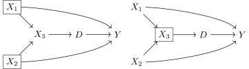
Figure 3.2: DAG with multiple solutions.

In this DAG in Figure 1.2, to identify the effect of \(D\) on \(Y\), we need to account for two backdoor paths:

1. Main causal path of interest

   1. \(D \rightarrow Y\)

2. Backdoor paths

   1. \(D\leftarrow X3\leftarrow X1 \rightarrow Y\) (backdoor path #1)

   2. \(D\leftarrow X3\leftarrow X2 \rightarrow Y\) (backdoor path #2)

To block these paths and identify the effect of \(D\) on \(Y\), we can either condition on \(X_3\) alone, which closes both paths because \(X_3\) is a noncollider, or we can condition on \(X_1\) and \(X_2\). We could also condition on all three variables, or combinations like \(X_1\) and \(X_3\). So, which strategy should you use, and why?

To illustrate this, I created a simulation.³ The ATE is equal to 1,000 and I assume constant treatment effects. I generated three variables, X1, X2, X3, that each reflected the previous DAG structure. I ran several regressions, each corresponding to a different control strategy from the DAG, and each summarized in Table [tab:multiple]. I repeated this process 1,000 times, resulting in 1,000 estimates for each strategy. The results are summarized in the table below.

No Controls	1149.706	23.29696
Condition on \(X_3\) only	999.4315	22.36062
Condition on \(X_2\) and \(X_3\)	999.9924	2.089094
Condition on \(X_1\) and \(X_3\)	999.9997	1.046352
Condition on \(X_1\) and \(X_2\)	999.9999	0.1033014
Condition on \(X_1\), \(X_2\), and \(X_3\)	999.9998	0.103288

The table shows the mean estimate and standard deviation for each conditioning strategy. Notice that all strategies yield estimates very close to the true effect of 1,000, confirming that they are unbiased. However, the standard deviations tell a different story. Conditioning on x3 alone has a standard deviation of 22.36, meaning it has a higher variability compared to other strategies. When conditioning on x1 and x2 the standard deviation drops significantly to 0.1033, indicating much higher precision.

Why is this the case? The reason is that x1 and x2 have significant impacts on earnings. Including them in the model reduces the residual variance, meaning the unexplained variation in earnings decreases, leaving only the random error term with a standard deviation of 5. In contrast, x3 alone doesn’t account for as much of the variation in earnings because it has actually no direct effect on it at all. It is simply a confounder along a chain of confounders connecting the treatment to the outcome. As such, when we only condition on it, while that is sufficient to correctly identify the ATE, it is not as precise as there is still a lot of variation in the outcome unaccounted for.

This illustrates that sometimes our choices in controlling for variables are not just about achieving unbiasedness. When variables are highly predictive of the potential outcomes, including them can reduce the variation in the outcome, allowing us to more precisely estimate the parameter of interest. This will be an important concept in later chapters as well.

3.3 Collider Bias

Sometimes colliders enter into the DAG in very subtle ways. To illustrate how, I will introduce two situations with simulations.

Movie Stars and Controlling for Colliders

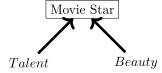
A 2009 CNN blog post that has since been taken down reported that the actress Megan Fox, who had recently starred in the movie Transformers, had been voted both the worst actress and most attractive actress of 2009 (Piazza 2009). While not explicit in the article, the implication was that talent and beauty were negatively correlated in the population—that is, that more attractive people were systematically less talented and vice versa. To illustrate the problems associated with conditioning on a collider, we will use this old blog post as our example to illustrate that conditioning on colliders can introduce biased estimates.⁴ Our example will be based on the following DAG:

Note that we have three variables: talent, beauty, and whether someone is a movie star. In this DAG, talent and beauty are not correlated—they are in fact independent. But, they both cause a person to become a movie star. For instance, maybe a large group of people in the population go to an audition. The casting director asks each of them to read, and then scores them on a scale measuring their beauty and their talent. People with high enough values for each become movie stars; the rest don’t. The paths associated with that narrative are:

1. Main causal path of interest

   1. Talent \(\rightarrow\) Beauty

2. Backdoor paths

   1. Talent \(\rightarrow\) Movie star \(\leftarrow\) Beauty (backdoor path #1)

Our DAG states that there is no causal effect of talent on beauty, but there is backdoor path from talent to beauty and it’s through movie star. But movie star is a collider, so there’s no threat from that backdoor path. If someone were to get their hands on a dataset containing information on a person’s talent, beauty, and their movie star status, and they wanted to test the hypothesis that talent had a negative effect on beauty, then they’d need only run this regression: \[ \begin{eqnarray} Beauty_i = \alpha + \delta Talent_i + \varepsilon_i \end{eqnarray} \tag{3.2}\] And \(\widehat{\delta}\) would capture the effect of talent on beauty in the population.

But without a DAG in hand, individuals might run this regression: \[ \begin{eqnarray} Beauty_i = \alpha + \delta Talent_i + \gamma Star_i + \varepsilon_i \end{eqnarray} \tag{3.3}\] And sadly, we know that if they run this regression, \(\widehat{\delta} \neq \delta\) because the \(Star_i\) variable is a collider. Let’s illustrate this with a simple program:

Stata Code

moviestar.do

clear all 
set seed 3444 

* 2500 independent draws from standard normal distribution 
set obs 2500 
generate beauty=rnormal() 
generate talent=rnormal() 

* Creating the collider variable (star) 
gen score=(beauty+talent) 
egen c85=pctile(score), p(85)   
gen star=(score>=c85) 
label variable star "Movie star" 

* Conditioning on the top 15\% 
twoway (scatter beauty talent, mcolor(black) msize(small) msymbol(smx)), ytitle(Beauty) xtitle(Talent) subtitle(Aspiring actors and actresses) by(star, total)

* Regressions
reg beauty talent
reg beauty talent star

R Code

moviestar.R

library(tidyverse)

set.seed(3444)

star_is_born <- tibble(
  beauty = rnorm(2500),
  talent = rnorm(2500),
  score = beauty + talent,
  c85 = quantile(score, .85),
  star = ifelse(score>=c85,1,0)
)

star_is_born %>% 
  lm(beauty ~ talent, .) %>% 
  ggplot(aes(x = talent, y = beauty)) +
  geom_point(size = 0.5, shape=23) + xlim(-4, 4) + ylim(-4, 4)

star_is_born %>% 
  filter(star == 1) %>% 
  lm(beauty ~ talent, .) %>% 
  ggplot(aes(x = talent, y = beauty)) +
  geom_point(size = 0.5, shape=23) + xlim(-4, 4) + ylim(-4, 4)

star_is_born %>% 
  filter(star == 0) %>% 
  lm(beauty ~ talent, .) %>% 
  ggplot(aes(x = talent, y = beauty)) +
  geom_point(size = 0.5, shape=23) + xlim(-4, 4) + ylim(-4, 4)

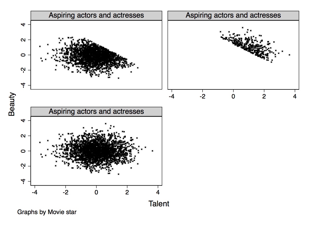
Figure 1.3 shows the output from this simulation. The bottom left panel shows the scatterplot between talent and beauty. Notice that the two variables are independent draws from the standard normal distribution, creating an oblong data cloud. But, because “movie star” is in the top 15 percentile of the distribution of a linear combination of talent and beauty, the movie star sample is formed by a frontier of the combined variables. This frontier has a negative slope and is in the upper right portion of the data cloud, creating a negative correlation between the observations in the movie star sample. Likewise, the collider bias has created a negative correlation between talent and beauty in the non-movie star sample as well. Yet we know that there is in fact no relationship between the two variables. This kind of sample selection creates spurious correlations. A random sample of the full population would be sufficient to show that there is no relationship between the two variables, but splitting the sample into movie stars only, we introduce spurious correlations between the two variables of interest.

Figure 3.3: Top left figure: Nonstar sample scatter plot of beauty (vertical axis) and talent (horizontal axis). Top right figure: Star sample scatter plot of beauty and talent. Bottom left figure: Entire (stars and nonstars combined) sample scatter plot of beauty and talent.

Now let’s see the coefficient estimates from the two regressions I mentioned. I’ve produced a table with the estimated coefficients from these two regression models in Table 3.1. Look at the coefficient on talent with and without movie star as a control. If we don’t include movie star, then the effect of talent on beauty is zero. But if we do include it, then the coefficient on talent because \(-0.276\) and is highly statistically significant.

Table 3.1: Regressions of Beauty on Talent with and Without Controlling for Movie Star

Dep var: Beauty
Talent	-0.007 (0.020)	-0.276*** | (0.019)
Movie star		1.67 (0.052)
N	2,500	2,500

Beauty and talent were both generated as random variables identical and independently drawn from the standard normal distribution. They are by construction independent of one another. The coefficient on talent has a \(p\)-value \(<0.001\).

Without a DAG, I don’t see how anyone in their right mind could resist running the regression for model (2). It just seems impossible to avoid because it’s simply so interesting. But the DAG says that doing so is dangerous because that DAG suggests talent and beauty both cause people to become movie stars, and thus controlling for that variable induces spurious correlations between talent and beauty, even in a simulation.

Discrimination and Collider Bias

Let’s examine a real world example around the problem of gender discrimination in labor markets. It is common to hear someone deny the existence of gender discrimination by saying that once occupation or other characteristics of a job are conditioned on, the wage disparity disappears or gets smaller. In other words, controlling for characteristics of the job, women received the same pay. But what if the occupation a person has is itself a consequence of discrimination? When would that be a collider?

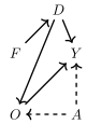
To illustrate, imagine the following simplified model. Assume that all women, for the sake of argument, are “treated” with discrimination and no men are. Firms respond in two ways: they pay them less, and they do not promote them, which means they get paid less. So two sources, in other words, of discrimination. Let me illustrate this with a DAG based on a simple occupational sorting model with unobserved heterogeneity: Notice that there is in fact no effect of females on earnings, because they are assumed to have identical productivity to males.

Thus if we could control for discrimination, we’d get a coefficient of zero as in this example because women are, initially, just as productive as men.⁵

But in this example, we aren’t interested in estimating the effect of female on earnings; we are interested in estimating the effect of discrimination itself. Now you can see several noticeable paths between discrimination and earnings. They are:

1. Main causal path of interest

   1. \(D \rightarrow Y\)

2. Backdoor paths

   1. \(D \rightarrow O \rightarrow Y\) (backdoor path #1)

   2. \(D \rightarrow O \leftarrow A \rightarrow Y\) (backdoor path #2)

The first path is not a backdoor path; rather it is a path whereby discrimination is mediated by occupation before it impacts earnings. In words, this would imply that women are discriminated against, which affects what jobs they hold, and as a result of those marginally worse jobs, are paid less. The second path relates to that channel, but is slightly more complicated. In this path, unobserved ability affects both which jobs people get as well as their earnings.

So let’s say we regress \(Y\) onto \(D\), our discrimination variable. This yields the total effect of discrimination as the weighted sum of both the direct effect of discrimination on earnings and the mediated effect of discrimination on earnings through occupational sorting.

But say that someone wants to control for occupation because they want to compare men and women in similar jobs. What then? Well, controlling for occupation in the regression closes down the mediation channel, but notice—it then opens up the second channel. Why? Because \(D \rightarrow O \leftarrow A \rightarrow Y\) has a collider \(O\). So when we control for occupation, we open up this second path. It had been closed because colliders close backdoor paths, but since we conditioned on it, we actually opened it instead. This is the reason we cannot merely control for occupation. Such a control ironically introduces new patterns of bias.⁶

What is needed rather is to control for occupation and ability, but since ability is unobserved, we cannot do that, and therefore we do not possess an identification strategy that satisfies the backdoor criterion. Let’s now look at code to illustrate this DAG.⁷ This simulation hard codes the data generating process represented by the previous DAG.

Stata Code

collider_discrimination.do

clear all 
set obs 10000 

* Half of the population is female. 
generate female = runiform()>=0.5 

* Innate ability is independent of gender. 
generate ability = rnormal() 

* All women experience discrimination. 
generate discrimination = female 

* Data generating processes.
generate occupation = (1) + (2)*ability + (0)*female + (-2)*discrimination + rnormal() 
generate wage = (1) + (-1)*discrimination + (1)*occupation + 2*ability + rnormal() 

* Regressions

regress wage discrimination 
regress wage discrimination occupation 
regress wage discrimination occupation ability

R Code

collider_discrimination.R

# Load necessary libraries
library(tidyverse)
library(stargazer)

# Data-generating process (DGP)
set.seed(123)
tb <- tibble(
  female = ifelse(runif(10000) >= 0.5, 1, 0),
  ability = rnorm(10000),
  discrimination = female,  # Discrimination linked to being female
  occupation = 1 + 2 * ability - 2 * discrimination + rnorm(10000),
  wage = 1 - discrimination + occupation + 2 * ability + rnorm(10000)
)

# Regressions
lm_1 <- lm(wage ~ female, tb)                          # Unconditional, biased
lm_2 <- lm(wage ~ female + occupation, tb)             # Conditional, still biased
lm_3 <- lm(wage ~ female + occupation + ability, tb)   # Fully conditional, unbiased

# Display results with stargazer
stargazer(lm_1, lm_2, lm_3, type = "text",
          column.labels = c("Unconditional (Biased)", 
                            "Conditional (Biased)", 
                            "Fully Conditional (Unbiased)"),
          dep.var.caption = "Dependent variable: Wage",
          omit.stat = c("f", "ser")) 

Notice that ability is a random variable without a parent in the system. Furthermore, notice that all women experience discrimination in this simulation. And then we have our last two generated variables: the heterogeneous occupations and their corresponding wages. Occupations are increasing in unobserved ability, but decreasing in discrimination. Wages are decreasing in discrimination but increasing in higher quality jobs and higher ability. Thus we know that discrimination exists in this simulation because we are hard coding it that way with the negative coefficients both the occupation and wage processes.

The regression coefficients from the three regressions at the end of the code are presented in Table 3.2. First note that when we simply regress wages onto gender, we get a large negative effect, which is the combination of the direct effect of discrimination on earnings and the indirect effect via occupation. But if we run the regression that Google and others recommend wherein we control for occupation, the sign on gender changes. It literally becomes positive! We know this is wrong because we hard coded the effect of gender to be \(-1\)! The problem is that occupation is a collider. It is caused by ability and discrimination.If we control for occupation, we open up a backdoor path between discrimination and earnings that is spurious and so strong it perverted the entire relationship. So only when we control for occupation and ability can we isolate the direct causal effect of gender on wages.

Table 3.2: Regressions Illustrating Confounding Bias with Simulated Gender Disparity

Covariates:	Biased unconditional	Biased	Unbiased conditional
Female	-3.074*** (0.000)	0.601*** (0.000)	-0.994*** (0.000)
Occupation		1.793*** (0.000)	0.991*** (0.000)
Ability			2.017*** (0.000)
N	10,000	10,000	10,000
Mean of dependent variable	0.45	0.45	0.45

3.4 Concluding Remarks

In conclusion, DAGs are powerful tools, not for creating reality, but for reflecting it in a structured and honest way. A good DAG is built on credible, good-faith knowledge of the phenomena your data represents. It demands that you become an expert in the context behind your data—the institutions, mechanisms, and processes that generate it. Without this deep understanding, choosing which variables to include or exclude becomes guesswork, which undermines the very purpose of the DAG.

A DAG’s value lies in its ability to guide your conditioning strategy—to help you isolate the source of randomness in your data and determine whether a causal effect can be identified. It doesn’t impose assumptions; it forces you to clarify and justify the ones you already hold. If used well, DAGs reveal the pathways to credible inference and illuminate where your design might falter.

To truly make DAGs work for you, embrace the process of learning the institutional details behind your data. Whether it’s visiting sites, conducting interviews, or collaborating with experts, this immersion allows you to construct DAGs that are grounded in the realities of the treatment assignment mechanism. As reflections of these mechanisms, DAGs can show you where the backdoor criterion might be satisfied—or where it may fail.

As we move into the next chapter, we’ll explore how DAGs interact with the potential outcomes framework, diving deeper into the conditioning strategies they inspire. For those wanting to go beyond what we’ve covered here, I encourage you to read Pearl, Glymour, and Jewell (2016) and Morgan and Winship (2014) for deeper insights into DAGs, and Imbens (2020) for a more critical perspective. These resources will reinforce your understanding and help you use DAGs to their fullest potential.

Angrist, Joshua D., and Jorn-Steffen Pischke. 2009. Mostly Harmless Econometrics. 1st ed. Princeton University Press.

Becker, Gary. 1994. Human Capital: A Theoretical and Empirical Analysis with Special Reference to Education. 3rd ed. University of Chicago Press.

Heckman, James, and Rodrigo Pinto. 2015. “Causal Analysis After Haavelmo.” Econometric Theory 31 (1): 115–51.

Imbens, Guido W. 2020. “Potential Outcome and Directed Acyclic Graph Approaches to Causality: Relevance for Empirical Practice in Economics.” Journal of Economic Literature 58 (4): 1129–79.

Matsueda, Ross L. 2012. “Handbook of Structural Equation Modeling.” In. Guilford Press.

Morgan, Stephen L., and Christopher Winship. 2014. Counterfactuals and Causal Inference: Methods and Principles for Social Research. 2nd ed. Cambridge University Press.

Pearl, Judea. 2009. Causality. 2nd ed. Cambridge University Press.

Pearl, Judea, Madelyn Glymour, and Nicholas P. Jewell. 2016. Causal Inference in Statistics: A Primer. Wiley.

Piazza, Jo. 2009. “Megan Fox Voted Worst - but Sexiest - Actress of 2009.” https://marquee.blogs.cnn.com/2009/12/30/megan-fox-voted-worst-but-sexiest-actress-of-2009/.

Wolpin, Kenneth I. 2013. The Limits of Inference Without Theory. MIT Press.

---

1. I will discuss the Wrights again in the chapter on instrumental variables. They were an interesting pair.

2. In the next chapter on unconfoundedness, we will explore regressions like this one, and other methods, in greater detail.

3. The code for this simulation is available at the online book but is suppressed for the sake of brevity.

4. I wish I had thought of this example, but alas, the sociologist Gabriel Rossman gets full credit.

5. Productivity could diverge, though, if women systematically sort down into lower quality occupations where human capital accumulates over time at a lower rate.

6. Angrist and Pischke (2009) talk about this problem in a different way, using language called “bad controls.” Bad controls are not merely conditioning on outcomes. Rather they are any situation where the outcome had been a collider linking the treatment to the outcome of interest, like \(D\) \(\rightarrow O \leftarrow A \rightarrow Y\).

7. The Stata code was written by the economist Erin Hengel.