Causal Inference:
The Mixtape.
Buy the print version today:
Buy the print version today:
My path to economics was not linear. I didn’t major in economics, for instance. I didn’t even take an economics course in college. I majored in English, for Pete’s sake. My ambition was to become a poet. But then I became intrigued with the idea that humans can form plausible beliefs about causal effects even without a randomized experiment. Twenty-five years ago, I wouldn’t have had a clue what that sentence even meant, let alone how to do such an experiment. So how did I get here? Maybe you would like to know how I got to the point where I felt I needed to write this book. The TL;DR version is that I followed a windy path from English to causal inference.1 First, I fell in love with economics. Then I fell in love with empirical research. Then I noticed that a growing interest in causal inference had been happening in me the entire time. But let me tell the longer version.
I majored in English at the University of Tennessee at Knoxville and graduated with a serious ambition to become a professional poet. But, while I had been successful writing poetry in college, I quickly realized that finding the road to success beyond that point was probably not realistic. I was newly married, with a baby on the way, and working as a qualitative research analyst doing market research. Slowly, I had stopped writing poetry altogether.2
My job as a qualitative research analyst was eye opening, in part because it was my first exposure to empiricism. My job was to do “grounded theory”—a kind of inductive approach to generating explanations of human behavior based on observations. I did this by running focus groups and conducting in-depth interviews, as well as through other ethnographic methods. I approached each project as an opportunity to understand why people did the things they did (even if what they did was buy detergent or pick a cable provider). While the job inspired me to develop my own theories about human behavior, it didn’t provide me a way of falsifying those theories.
I lacked a background in the social sciences, so I would spend my evenings downloading and reading articles from the Internet. I don’t remember how I ended up there, but one night I was on the University of Chicago Law and Economics working paper series website when a speech by Gary Becker caught my eye. It was his Nobel Prize acceptance speech on how economics applies to all of human behavior (Becker 1993), and reading it changed my life. I thought economics was about stock markets and banks until I read that speech. I didn’t know economics was an engine that one could use to analyze all of human behavior. This was overwhelmingly exciting, and a seed had been planted.
But it wasn’t until I read an article on crime by Lott and Mustard (1997) that I became truly enamored of economics. I had no idea that there was an empirical component where economists sought to estimate causal effects with quantitative data. A coauthor of that paper was David Mustard, then an associate professor of economics at the University of Georgia, and one of Gary Becker’s former students. I decided that I wanted to study with Mustard, and so I applied to the University of Georgia’s doctoral program in economics. I moved to Athens, Georgia, with my wife, Paige, and our infant son, Miles, and started classes in the fall of 2002.
After passing my first-year comprehensive exams, I took Mustard’s labor economics field class and learned about a variety of topics that would shape my interests for years. These topics included the returns to education, inequality, racial discrimination, crime, and many other fascinating topics in labor. We read many, many empirical papers in that class, and afterwards I knew that I would need a strong background in econometrics to do the kind of research I cared about. In fact, I decided to make econometrics my main field of study. This led me to work with Christopher Cornwell, an econometrician and labor economist at Georgia. I learned a lot from Chris, both about econometrics and about research itself. He became a mentor, coauthor, and close friend.
Econometrics was difficult. I won’t even pretend I was good at it. I took all the econometrics courses offered at the University of Georgia, some more than once. They included classes covering topics like probability and statistics, cross-sections, panel data, time series, and qualitative dependent variables. But while I passed my field exam in econometrics, I struggled to understand econometrics at a deep level. As the saying goes, I could not see the forest for the trees. Something just wasn’t clicking.
I noticed something, though, while I was writing the third chapter of my dissertation that I hadn’t noticed before. My third chapter was an investigation of the effect of abortion legalization on the cohort’s future sexual behavior (Cunningham and Cornwell 2013). It was a revisiting of Donohue and Levitt (2001). One of the books I read in preparation for my study was Levine (2004), which in addition to reviewing the theory of and empirical studies on abortion had a little table explaining the difference-in-differences identification strategy. The University of Georgia had a traditional econometrics pedagogy, and most of my field courses were theoretical (e.g., public economics, industrial organization), so I never really had heard the phrase “identification strategy,” let alone “causal inference.” Levine’s simple difference-in-differences table for some reason opened my eyes. I saw how econometric modeling could be used to isolate the causal effects of some treatment, and that led to a change in how I approach empirical problems.
My first job out of graduate school was as an assistant professor at Baylor University in Waco, Texas, where I still work and live today. I was restless the second I got there. I could feel that econometrics was indispensable, and yet I was missing something. But what? It was a theory of causality. I had been orbiting that theory ever since seeing that difference-in-differences table in Levine (2004). But I needed more. So, desperate, I did what I always do when I want to learn something new—I developed a course on causality to force myself to learn all the things I didn’t know.
I named the course Causal Inference and Research Design and taught it for the first time to Baylor master’s students in 2010. At the time, I couldn’t really find an example of the sort of class I was looking for, so I cobbled together a patchwork of ideas from several disciplines and authors, like labor economics, public economics, sociology, political science, epidemiology, and statistics. You name it. My class wasn’t a pure econometrics course; rather, it was an applied empirical class that taught a variety of contemporary research designs, such as difference-in-differences, and it was filled with empirical replications and readings, all of which were built on the robust theory of causality found in Donald Rubin’s work as well as the work of Judea Pearl. This book and that class are in fact very similar to one another.3
So how would I define causal inference? Causal inference is the leveraging of theory and deep knowledge of institutional details to estimate the impact of events and choices on a given outcome of interest. It is not a new field; humans have been obsessing over causality since antiquity. But what is new is the progress we believe we’ve made in estimating causal effects both inside and outside the laboratory. Some date the beginning of this new, modern causal inference to Fisher (1935), Haavelmo (1943), or Rubin (1974). Some connect it to the work of early pioneers like John Snow. We should give a lot of credit to numerous highly creative labor economists from the late 1970s to late 1990s whose ambitious research agendas created a revolution in economics that continues to this day. You could even make an argument that we owe it to the Cowles Commission, Philip and Sewall Wright, and the computer scientist Judea Pearl.
But however you date its emergence, causal inference has now matured into a distinct field, and not surprisingly, you’re starting to see more and more treatments of it as such. It’s sometimes reviewed in a lengthy chapter on “program evaluation” in econometrics textbooks (Wooldridge 2010), or even given entire book-length treatments. To name just a few textbooks in the growing area, there’s Angrist and Pischke (2009), Morgan and Winship (2014), Guide W. Imbens and Rubin (2015), and probably a half dozen others, not to mention numerous, lengthy treatments of specific strategies, such as those found in Angrist and Krueger (2001) and Guido W. Imbens and Lemieux (2008). The market is quietly adding books and articles about identifying causal effects with data all the time.
So why does Causal Inference: The Mixtape exist? Well, to put it bluntly, a readable introductory book with programming examples, data, and detailed exposition didn’t exist until this one. My book is an effort to fill that hole, because I believe what researchers really need is a guide that takes them from knowing almost nothing about causal inference to a place of competency. Competency in the sense that they are conversant and literate about what designs can and cannot do. Competency in the sense that they can take data, write code and, using theoretical and contextual knowledge, implement a reasonable design in one of their own projects. If this book helps someone do that, then this book will have had value, and that is all I can and should hope for.
But what books out there do I like? Which ones have inspired this book? And why don’t I just keep using them? For my classes, I mainly relied on Morgan and Winship (2014), Angrist and Pischke (2009), as well as a library of theoretical and empirical articles. These books are in my opinion definitive classics. But they didn’t satisfy my needs, and as a result, I was constantly jumping between material. Other books were awesome but not quite right for me either. Guide W. Imbens and Rubin (2015) cover the potential outcomes model, experimental design, and matching and instrumental variables, but not directed acyclic graphical models (DAGs), regression discontinuity, panel data, or synthetic control. Morgan and Winship (2014) cover DAGs, the potential outcomes model, and instrumental variables, but have too light a touch on regression discontinuity and panel data for my tastes. They also don’t cover synthetic control, which has been called the most important innovation in causal inference of the last 15 years by Athey and Imbens (2017). Angrist and Pischke (2009) is very close to what I need but does not include anything on synthetic control or on the graphical models that I find so critically useful. But maybe most importantly, Guide W. Imbens and Rubin (2015), Angrist and Pischke (2009), and Morgan and Winship (2014) do not provide any practical programming guidance, and I believe it is in replication and coding that we gain knowledge in these areas.4
This book was written with a few different people in mind. It was written first and foremost for practitioners, which is why it includes easy-to-download data sets and programs. It’s why I have made several efforts to review papers as well as replicate the models as much as possible. I want readers to understand this field, but as important, I want them to feel empowered so that they can use these tools to answer their own research questions.
Another person I have in mind is the experienced social scientist who wants to retool. Maybe these are people with more of a theoretical bent or background, or maybe they’re people who simply have some holes in their human capital. This book, I hope, can help guide them through the modern theories of causality so common in the social sciences, as well as provide a calculus in directed acyclic graphical models that can help connect their knowledge of theory with estimation. The DAGs in particular are valuable for this group, I think.
A third group that I’m focusing on is the nonacademic person in industry, media, think tanks, and the like. Increasingly, knowledge about causal inference is expected throughout the professional world. It is no longer simply something that academics sit around and debate. It is crucial knowledge for making business decisions as well as for interpreting policy.
Finally, this book is written for people very early in their careers, be they undergraduates, graduate students, or newly minted PhDs. My hope is that this book can give them a jump start so that they don’t have to meander, like many of us did, through a somewhat labyrinthine path to these methods.
It is very common these days to hear someone say “correlation does not mean causality.” Part of the purpose of this book is to help readers be able to understand exactly why correlations, particularly in observational data, are unlikely to be reflective of a causal relationship. When the rooster crows, the sun soon after rises, but we know the rooster didn’t cause the sun to rise. Had the rooster been eaten by the farmer’s cat, the sun still would have risen. Yet so often people make this kind of mistake when naively interpreting simple correlations.

But weirdly enough, sometimes there are causal relationships between two things and yet no observable correlation. Now that is definitely strange. How can one thing cause another thing without any discernible correlation between the two things? Consider this example, which is illustrated in Figure 1.1. A sailor is sailing her boat across the lake on a windy day. As the wind blows, she counters by turning the rudder in such a way so as to exactly offset the force of the wind. Back and forth she moves the rudder, yet the boat follows a straight line across the lake. A kindhearted yet naive person with no knowledge of wind or boats might look at this woman and say, “Someone get this sailor a new rudder! Hers is broken!” He thinks this because he cannot see any relationship between the movement of the rudder and the direction of the boat.
But does the fact that he cannot see the relationship mean there isn’t one? Just because there is no observable relationship does not mean there is no causal one. Imagine that instead of perfectly countering the wind by turning the rudder, she had instead flipped a coin—heads she turns the rudder left, tails she turns the rudder right. What do you think this man would have seen if she was sailing her boat according to coin flips? If she randomly moved the rudder on a windy day, then he would see a sailor zigzagging across the lake. Why would he see the relationship if the movement were randomized but not be able to see it otherwise? Because the sailor is endogenously moving the rudder in response to the unobserved wind. And as such, the relationship between the rudder and the boat’s direction is canceled—even though there is a causal relationship between the two.
This sounds like a silly example, but in fact there are more serious versions of it. Consider a central bank reading tea leaves to discern when a recessionary wave is forming. Seeing evidence that a recession is emerging, the bank enters into open-market operations, buying bonds and pumping liquidity into the economy. Insofar as these actions are done optimally, these open-market operations will show no relationship whatsoever with actual output. In fact, in the ideal, banks may engage in aggressive trading in order to stop a recession, and we would be unable to see any evidence that it was working even though it was!
Human beings engaging in optimal behavior are the main reason correlations almost never reveal causal relationships, because rarely are human beings acting randomly. And as we will see, it is the presence of randomness that is crucial for identifying causal effect.
Buy the print version today:
Certain presentations of causal inference methodologies have sometimes been described as atheoretical, but in my opinion, while some practitioners seem comfortable flying blind, the actual methods employed in causal designs are always deeply dependent on theory and local institutional knowledge. It is my firm belief, which I will emphasize over and over in this book, that without prior knowledge, estimated causal effects are rarely, if ever, believable. Prior knowledge is required in order to justify any claim of a causal finding. And economic theory also highlights why causal inference is necessarily a thorny task. Let me explain.
There’s broadly thought to be two types of data. There’s experimental data and non-experimental data. The latter is also sometimes called observational data. Experimental data is collected in something akin to a laboratory environment. In a traditional experiment, the researcher participates actively in the process being recorded. It’s more difficult to obtain data like this in the social sciences due to feasibility, financial cost, or moral objections, although it is more common now than was once the case. Examples include the Oregon Medicaid Experiment, the RAND health insurance experiment, the field experiment movement inspired by Esther Duflo, Michael Kremer, Abhijit Banerjee, and John List, and many others.
Observational data is usually collected through surveys in a retrospective manner, or as the by-product of some other business activity (“big data”). In many observational studies, you collect data about what happened previously, as opposed to collecting data as it happens, though with the increased use of web scraping, it may be possible to get observational data closer to the exact moment in which some action occurred. But regardless of the timing, the researcher is a passive actor in the processes creating the data itself. She observes actions and results but is not in a position to interfere with the environment in which the units under consideration exist. This is the most common form of data that many of us will ever work with.
Economic theory tells us we should be suspicious of correlations found in observational data. In observational data, correlations are almost certainly not reflecting a causal relationship because the variables were endogenously chosen by people who were making decisions they thought were best. In pursuing some goal while facing constraints, they chose certain things that created a spurious correlation with other things. And we see this problem reflected in the potential outcomes model itself: a correlation, in order to be a measure of a causal effect, must be based on a choice that was made independent of the potential outcomes under consideration. Yet if the person is making some choice based on what she thinks is best, then it necessarily is based on potential outcomes, and the correlation does not remotely satisfy the conditions we need in order to say it is causal. To put it as bluntly as I can, economic theory says choices are endogenous, and therefore since they are, the correlations between those choices and outcomes in the aggregate will rarely, if ever, represent a causal effect.
Now we are veering into the realm of epistemology. Identifying causal effects involves assumptions, but it also requires a particular kind of belief about the work of scientists. Credible and valuable research requires that we believe that it is more important to do our work correctly than to try and achieve a certain outcome (e.g., confirmation bias, statistical significance, asterisks). The foundations of scientific knowledge are scientific methodologies. True scientists do not collect evidence in order to prove what they want to be true or what others want to believe. That is a form of deception and manipulation called propaganda, and propaganda is not science. Rather, scientific methodologies are devices for forming a particular kind of belief. Scientific methodologies allow us to accept unexpected, and sometimes undesirable, answers. They are process oriented, not outcome oriented. And without these values, causal methodologies are also not believable.
One of the cornerstones of scientific methodologies is empirical analysis.5 By empirical analysis, I mean the use of data to test a theory or to estimate a relationship between variables. The first step in conducting an empirical economic analysis is the careful formulation of the question we would like to answer. In some cases, we would like to develop and test a formal economic model that describes mathematically a certain relationship, behavior, or process of interest. Those models are valuable insofar as they both describe the phenomena of interest and make falsifiable (testable) predictions. A prediction is falsifiable insofar as we can evaluate, and potentially reject, the prediction with data.6 A model is the framework with which we describe the relationships we are interested in, the intuition for our results, and the hypotheses we would like to test.7
After we have specified a model, we turn it into what is called an econometric model, which can be estimated directly with data. One clear issue we immediately face is regarding the functional form of the model, or how to describe the relationships of the variables we are interested in through an equation. Another important issue is how we will deal with variables that cannot be directly or reasonably observed by the researcher, or that cannot be measured very well, but which play an important role in our model.
A generically important contribution to our understanding of causal inference is the notion of comparative statics. Comparative statics are theoretical descriptions of causal effects contained within the model. These kinds of comparative statics are always based on the idea of ceteris paribus—or “all else constant.” When we are trying to describe the causal effect of some intervention, for instance, we are always assuming that the other relevant variables in the model are not changing. If they were changing, then they would be correlated with the variable of interest and it would confound our estimation.8
To illustrate this idea, let’s begin with a basic economic model: supply and demand equilibrium and the problems it creates for estimating the price elasticity of demand. Policy-makers and business managers have a natural interest in learning the price elasticity of demand because knowing it enables firms to maximize profits and governments to choose optimal taxes, and whether to restrict quantity altogether (Becker, Grossman, and Murphy 2006). But the problem is that we do not observe demand curves, because demand curves are theoretical objects. More specifically, a demand curve is a collection of paired potential outcomes of price and quantity. We observe price and quantity equilibrium values, not the potential price and potential quantities along the entire demand curve. Only by tracing out the potential outcomes along a demand curve can we calculate the elasticity.
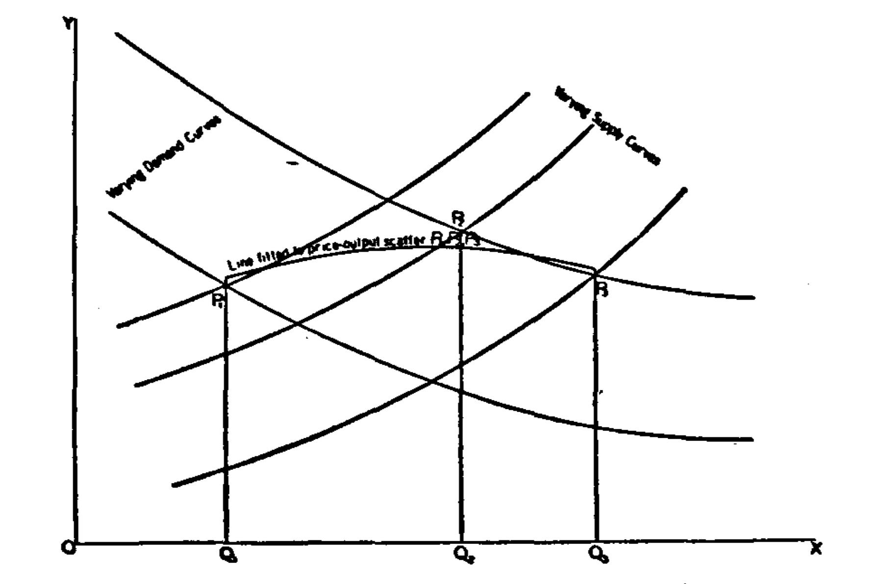
To see this, consider this graphic from Philip Wright’s Appendix B (Wright 1928), which we’ll discuss in greater detail later (Figure 1.2). The price elasticity of demand is the ratio of percentage changes in quantity to price for a single demand curve. Yet, when there are shifts in supply and demand, a sequence of quantity and price pairs emerges in history that reflect neither the demand curve nor the supply curve. In fact, connecting the points does not reflect any meaningful or useful object.
The price elasticity of demand is the solution to the following equation:
\[ \epsilon = \frac{\partial \log Q}{\partial \log P} \]
But in this example, the change in \(P\) is exogenous. For instance, it holds supply fixed, the prices of other goods fixed, income fixed, preferences fixed, input costs fixed, and so on. In order to estimate the price elasticity of demand, we need changes in \(P\) that are completely and utterly independent of the otherwise normal determinants of supply and the other determinants of demand. Otherwise we get shifts in either supply or demand, which creates new pairs of data for which any correlation between \(P\) and \(Q\) will not be a measure of the elasticity of demand.
The problem is that the elasticity is an important object, and we need to know it, and therefore we need to solve this problem. So given this theoretical object, we must write out an econometric model as a starting point. One possible example of an econometric model would be a linear demand function:
\[ \log Q_d = \alpha+\delta \log P+\gamma X + u \]
where \(\alpha\) is the intercept, \(\delta\) is the elasticity of demand, \(X\) is a matrix of factors that determine demand like the prices of other goods or income, \(\gamma\) is the coefficient on the relationship between \(X\) and \(Q_d\), and \(u\) is the error term.9
Foreshadowing the content of this mixtape, we need two things to estimate price elasticity of demand. First, we need numerous rows of data on price and quantity. Second, we need for the variation in price in our imaginary data set to be independent of \(u\). We call this kind of independence exogeneity. Without both, we cannot recover the price elasticity of demand, and therefore any decision that requires that information will be based on stabs in the dark.
This book is an introduction to research designs that can recover causal effects. But just as importantly, it provides you with hands-on practice to implement these designs. Implementing these designs means writing code in some type of software. I have chosen to illustrate these designs using two popular software languages: Stata (most commonly used by economists) and R (most commonly used by everyone else).
The book contains numerous empirical exercises illustrated in the Stata and R programs. These exercises are either simulations (which don’t need external data) or exercises requiring external data. The data needed for the latter have been made available to you at Github. The Stata examples will download files usually at the start of the program using the following command: use https://github.com/scunning1975/mixtape/raw/master/DATAFILENAME.DTA, where DATAFILENAME.DTA is the name of a particular data set.
For R users, it is a somewhat different process to load data into memory. In an effort to organize and clean the code, my students Hugo Sant’Anna and Terry Tsai created a function to simplify the data download process. This is partly based on a library called haven, which is a package for reading data files. It is secondly based on a set of commands that create a function that will then download the data directly from Github.10
Some readers may not be familiar with either Stata or R but nonetheless wish to follow along. I encourage you to use this opportunity to invest in learning one or both of these languages. It is beyond the scope of this book to provide an introduction to these languages, but fortunately, there are numerous resources online. For instance, Christopher Baum has written an excellent introduction to Stata at http://fmwww.bc.edu/GStat/docs/IntroStata.pdf. Stata is popular among microeconomists, and given the amount of coauthoring involved in modern economic research, an argument could be made for investing in it solely for its ability to solve basic coordination problems between you and potential coauthors. But a downside to Stata is that it is proprietary and must be purchased. And for some people, that may simply be too big of a barrier—especially for anyone simply wanting to follow along with the book. R on the other hand is open-source and free. Tutorials on Basic R can be found at https://cran.r-project.org/doc/contrib/Paradis-rdebuts_en.pdf, and an introduction to Tidyverse (which is used throughout the R programming) can be found at https://r4ds.had.co.nz. Using this time to learn R would likely be well worth your time.
Perhaps you already know R and want to learn Stata. Or perhaps you know Stata and want to learn R. Then this book may be helpful because of the way in which both sets of code are put in sequence to accomplish the same basic tasks. But, with that said, in many situations, although I have tried my best to reconcile results from Stata and R, I was not always able to do so. Ultimately, Stata and R are different programming languages that sometimes yield different results because of different optimization procedures or simply because the programs are built slightly differently. This has been discussed occasionally in articles in which authors attempt to better understand what accounts for the differing results. I was not always able to fully reconcile different results, and so I offer the two programs as simply alternative approaches. You are ultimately responsible for anything you do on your own using either language for your research. I leave it to you ultimately to understand the method and estimating procedure contained within a given software and package.
In conclusion, simply finding an association between two variables might be suggestive of a causal effect, but it also might not. Correlation doesn’t mean causation unless key assumptions hold. Before we start digging into the causal methodologies themselves, though, I need to lay down a foundation in statistics and regression modeling. Buckle up! This is going to be fun.
Buy the print version today:
“Too long; didn’t read.”↩︎
Rilke said you should quit writing poetry when you can imagine yourself living without it (Rilke 2012). I could imagine living without poetry, so I took his advice and quit. Interestingly, when I later found economics, I went back to Rilke and asked myself if I could live without it. This time, I decided I couldn’t, or wouldn’t—I wasn’t sure which. So I stuck with it and got a PhD.↩︎
I decided to write this book for one simple reason: I didn’t feel that the market had provided the book that I needed for my students. So I wrote this book for my students and me so that we’d all be on the same page. This book is my best effort to explain causal inference to myself. I felt that if I could explain causal inference to myself, then I would be able to explain it to others too. Not thinking the book would have much value outside of my class, I posted it to my website and told people about it on Twitter. I was surprised to learn that so many people found the book helpful.↩︎
Although Angrist and Pischke (2009) provides an online data warehouse from dozens of papers, I find that students need more pedagogical walk-throughs and replications for these ideas to become concrete and familiar.↩︎
It is not the only cornerstone, or even necessarily the most important cornerstone, but empirical analysis has always played an important role in scientific work.↩︎
You can also obtain a starting point for empirical analysis through an intuitive and less formal reasoning process. But economics favors formalism and deductive methods.↩︎
Scientific models, be they economic ones or otherwise, are abstract, not realistic, representations of the world. That is a strength, not a weakness. George Box, the statistician, once quipped that “all models are wrong, but some are useful.” A model’s usefulness is its ability to unveil hidden secrets about the world. No more and no less.↩︎
One of the things implied by ceteris paribus that comes up repeatedly in this book is the idea of covariate balance. If we say that everything is the same except for the movement of one variable, then everything is the same on both sides of that variable’s changing value. Thus, when we invoke ceteris paribus, we are implicitly invoking covariate balance—both the observable and the unobservable covariates.↩︎
More on the error term later.↩︎
This was done solely for aesthetic reasons. Often the URL was simply too long for the margins of the book otherwise.↩︎